Elementary discrete mathematics
Table of contents
- Front page
- Summer I 2020 syllabus
- Problems
- 0. What is discrete mathematics?
- PART 1: SETS AND LOGIC
- Part 1 videos
- 1. Sets
- 2. Propositional logic
- 3. Predicate logic
- PART 2: PROOF AND RECURSION
- Part 2 videos
- 4. Proofs
- 5. Recursion and integer representation
- 6. Sequences and sums
- 7. Asymptotics
- 8. Proof by induction
- INTERLUDE
- PART 3: COMBINATORICS
- 9. Introduction to combinatorics
- 10. Ordered samples
- 11. Unordered samples
- 12. Multinomial coefficients
- 13. Probability
- PART 4: RELATIONS
- 14. Boolean matrices
- 15. Relations
- 16. Closure and composition
- 17. Equivalence relations
- 18. Partial orders
- EPILOGUE
0. What is discrete mathematics?
0.1 It’s math you do quietly, right?
The phrase “discrete mathematics” is often used nebulously to refer to a certain branch of mathematics that, from the college point of view, is “not calculus” or perhaps is applicable to computer science. In this section, we will try to understand what it means for a topic to fall under the umbrella of discrete mathematics.
0.2 But really, what is it?
Here’s a question: What is the next number after ? Your answer depends on “where you live,” so to speak. If you live in the rational numbers (numbers that can be expressed as fractions, like ) or the real numbers (including numbers that can’t be written as fractions, like ), you can’t answer the question. If you give be a real or a rational number that’s a little more than , say , I can find something even smaller; say, .
If you live in the set of natural numbers, which is the set of numbers that are useful for counting things in the world, the question does have an answer: . The natural numbers do not suffer from the crowding issue that the rationals and the real do; all of their elements are sufficiently “far apart” in this way. There is , and then , and nothing in between. In this sense they are discrete. In this book, we will (usually) live in the natural numbers.
0.3 Some examples
Here are some questions we might try to answer using discrete mathematics. In fact, you will be able to answer all these questions by the end of the book.
Suppose we have a program that will activate condition 4 if conditions 1 and 2 are met but not condition 3. How do we know when condition 4 is active?
We can use logic to represent this program with the statement , and then use truth tables to determine exactly when condition 4 will trigger.
Which of these two programs is more efficient?
A sequence is a function of natural numbers. An example is the number of steps it takes to run a computer program with inputs. If grows must faster than does, that can tell us that one program scales worse for large quantities of data.
Some members of a community are sick. How do we know who is at risk of being infected?
Relations encode relationships between sets of objects. We may compose relations to iterate those relationships over and over again. If person is sick and has come into contact with person , and has come into contact with person , and has since seen , then is at risk.
0.4 How to use this book
Chapters 1-8 must be done in order. Each chapter has a section of exercises located on the problems page. These exercises should be attempted after each chapter. If you are in MATH 174 at Coastal Carolina University, these exercises are your homework.
Then, chapters 9-13 (on combinatorics) and chapters 14-18 (on relations) may be attempted in that order, or in the order 14-18; 9-13. Be aware that some of the exercises in 14-18 assume that the reader has learned the combinatorial material. So, if you follow the alternate order, leave these exercises for later.
This book is paired with a four playlists on my YouTube channel. Playlist 1 (sets and logic) maps to chapters 1-3, playlist 2 (proof and recursion) maps to chapters 4-8, playlist 3 (combinatorics) maps to chapters 9-13, and playlist 4 (relations) maps to chapters 14-18.
These videos are very short demonstrations and examples of the material pursued in depth by the book. I am not sure which ordering is better: book then videos, or videos then book. Choose your own adventure.
I try to use the invitational “we” throughout the book and maintain some level of formality, but sometimes my annoying authorial voice pokes through. I apologize if that bothers you.
Each chapter ends with several “takeaways” that summarize the chapter. Starting with the fourth chapter, if necessary, each chapter begins with hint to go back and look at some things you may not have thought about in a while.
0.5 The point of this book
– is to teach you discrete mathematics, of course.
But much more broadly, this book is intended to teach you to think mathematically. You may be a student who has never seen any math beyond calculus or algebra, or perhaps you dread doing math. The point of this book is to get you to learn to think deeply, communicate carefully, and not shy away from difficult material.
As you proceed, have something to write with on hand. Work each example along with the book. Then, at the end of each chapter, work the exercises. Some are more difficult than others, but are well worth doing to improve your understanding. Work along with someone at roughly your skill level, share solutions and ask each other questions.
Everyone can be a “math person!” So, let’s get started.
1. Sets
Videos:
1.1 Membership
For nearly all interested parties, sets form the foundation of all mathematics. Every mathematical objects you have ever encountered can be described as a set, from numbers themselves to functions and matrices.
We will say that a set is an unordered collection of objects, called its elements. When is an element of the set , we write .
Examples. Our starting point will be the set of all natural numbers,
Certain sets are special enough to get their own names, with bold or “blackboard bold” face. Sometimes (especially in ink) you will see instead. Note that the elements of the set are enclosed in curly braces. Proper notation is not optional; using the wrong notation is like saying “milk went store” to mean “I went to the store to get milk.” Finally, not everyone agrees that is a natural number, but computer scientists do.
If we take and include its negatives, we get the integers
Notice that in the case of an infinite set, or even a large finite set, we can use ellipses when a pattern is established. One infinite set that defies a pattern is the set of prime numbers. You may recall that a prime number is a positive integer with exactly two factors: itself and . We may list a few: but there is no pattern that allows us to employ ellipses.
Fortunately there is another way to write down a set. All previous examples have used roster notation, where the elements are simply listed. It may be more convenient to use set-builder notation, where the set is instead described with a rule that exactly characterizes this element. In that case, the set of primes can be written as
To provide one last example, consider the set of all U.S. states. In roster notation this set is a nightmare: {AL, AK, AZ, AR, CA, CO, CT, DE, FL, GA, HI, ID, IL, IN, IA, KS, KY, LA, ME, MD, MA, MI, MN, MS, MO, MT, NE, NV, NH, NJ, NM, NY, NC, ND, OH, OK, OR, PA, RI, SC, SD, TN, TX, UT, VT, VA, WA, WV, WI, WY}. But in set-builder notation we simply write
Definition 1.1.1. Two sets and are equal if they contain exactly the same elements, in which case we write .
Remember that sets are unordered, so even .
Definition 1.1.2. Let be a finite set. Its cardinality, denoted , is the number of elements in .
Example. If , then .
We can talk about the cardinality of infinite sets, but that is far beyond the scope of this course.
1.2 Containment
One of the most important ideas when dealing with sets is that of a subset.
Definition 1.2.1. Let and be sets. We say is a subset of if every element of is also an element of .
Examples. Put , , and . Then , , but and .
In mathematics, true statements are either definitions (those taken for granted) or theorems (those proven from the definitions). We will learn to prove more difficult theorems later, but for now we can prove a simple one.
Theorem 1.2.2. Every set is a subset of itself.
A proof is simply an argument that convinces its reader of the truth of a mathematical fact. Valid proofs must only use definitions and the hypotheses of the theorem; it is not correct to assume more than you are given. So the ingredients in the proof of this theorem are simply going to be a set and the definition of the word “subset.”
Proof. Let be a set. Suppose is an arbitrary element of . Then, is also an element of . Because was shown to have any arbitrary element of , then .
Notice that the actual make-up of the set is irrelevant. If has an element, then also has that element, and that is all it takes to conclude . It would be incorrect to try to prove from an example: just because is a subset of itself doesn’t necessarily mean that is!
We will discuss logic and proof-writing at length as we continue. For now, let’s continue learning about sets and proving the “simple” theorems as we go.
Definition 1.2.3. The set with no elements is called the empty set, denoted or .
With a little logical sleight-of-hand, we can prove another (much more surprising) theorem.
Theorem 1.2.4. The empty set is a subset of every set.
Proof. Let be a set. We may conclude if every element of is an element of . Observe that this statement is equivalent to saying that no elements of are not elements of . Because there are no elements of at all, this statement is true; and we are done.
Perhaps you already agree with the central claim of the proof, that there are no difference between the statements "everything in is in " and "nothing in is not in ". If you do not, take it on faith for now. When we study predicate logic later you will have the tools to convince yourself of the claim.
Such a statement that relies on the emptiness of is said to be vacuously true.
When , we say contains or that is a superset of . With the idea of containment in hand we can construct a new type of set.
Definition 1.2.5. Let be a set. Its power set is the set whose elements are the subsets of . That is,
Wait - our elements are sets? Yes, and this is perfectly fine! Elements can be all sorts of things, other sets included. When we have a “set of sets” we typically refer to it as a family or a collection to avoid using the same word and over and over.
Example. Let . Then
Notice that the number of sets in can be derived from the number of elements in .
Theorem 1.2.6. If is finite, then .
We will come back to prove this theorem much later, once we have learned how to count!
1.3 The algebra of sets
You are used to word “algebra” as it refers to a class where you must solve some equations for . If you think about those classes, they are really about understanding operations and functions of real numbers. Think about it: a successful algebra student will know how to manipulate sums, products, polynomials, roots, and exponential functions – ways of combining and mapping real numbers.
So, “algebra” in general refers to the ways objects may be combined and mapped. In this section, we will see many ways that sets can be combined to produce new sets.
Definition 1.3.1. Let and be sets. Their union is the set of all elements that are in at least one of or ; in set builder notation this is
Definition 1.3.2. Let and be sets. Their intersection is the set of all elements that are in both and ; in set builder notation this is
A useful way to visualize combinations of sets is with a Venn diagram. The Venn diagrams for union and intersection are shown below.
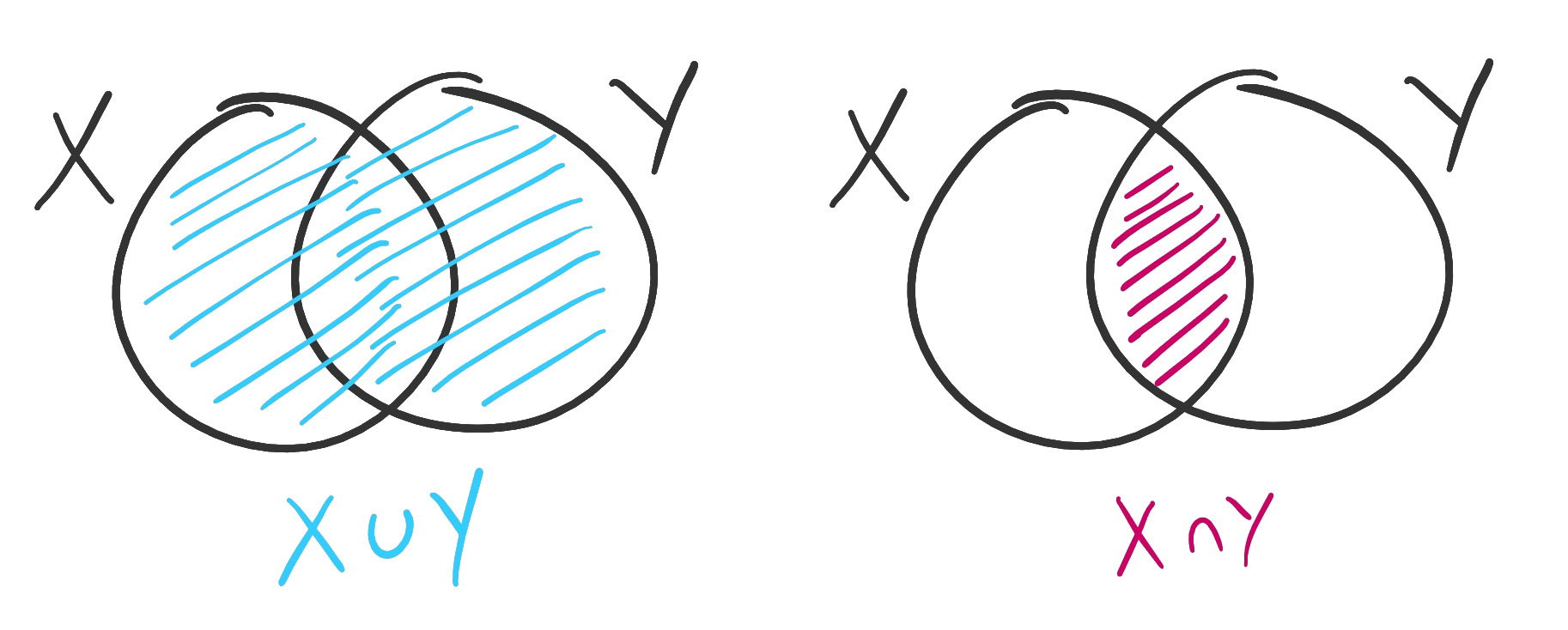
Figure. On the left, the union of two sets; on the right, the intersection.
Example. Let and . Their union is
and their intersection is Notice that we do not repeat elements in a set. An element is either in the set or it isn’t. (A generalization, the multiset, will be developed in Chapter 11.) Therefore, (recall, the number of elements in the union) won’t just be .
Theorem 1.3.3. If and are finite sets, then
Proof. If an element is only in , it will be counted by . If an element is only in , it will be counted by . Therefore any elements in will be counted twice. There are exactly of these elements, so subtracting that amount gives .
Definition 1.3.4. Let and be sets. The difference is the set of all elements in but not ; i.e.
Example. Like before, let and . Then . Notice that ; just like with numbers, taking a diference is not commutative. (That is, the order matters.)
Often when working with sets there is a universal or ambient set, sometimes denoted , that all of our sets are assumed to be subsets of. This set is typically inferred from context.
- In calculus, this set might be .
- If my set is “students taking MATH 174,” my universal set might be the set of all students at Coastal Carolina.
- In probability theory, the sets are events (e.g. “the roll is odd”) and is the sample space (e.g. all possible rolls of the die).
Definition 1.3.5. Let be a set contained in some universal set . The complement of (relative to ), denoted , is all the elements not in . In other words, .
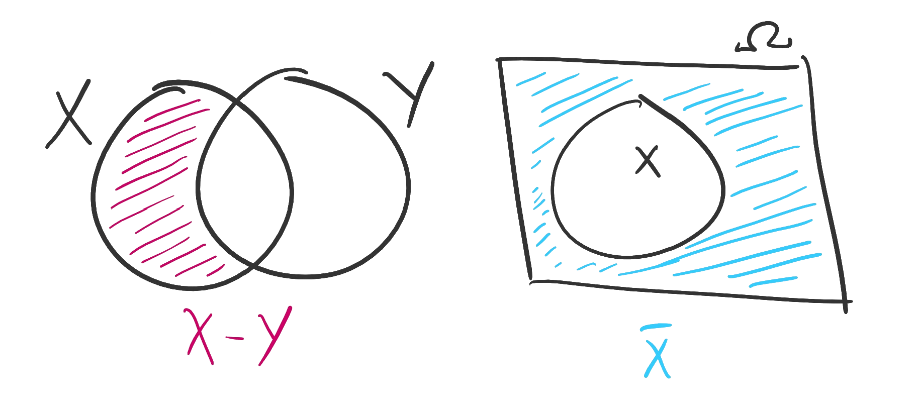
Figure. On the left, the difference of two sets shaded in pink. On the right, the complement of a set shaded in blue.
Example. Suppose is contained in the universal set . Then .
Definition 1.3.6. Let and be sets. Their Cartesian product (in this book, just “product”) is the set The elements of the product are called ordered pairs.
As the name implies, the ordering of the entries in an ordered pair matters. Therefore, we will adopt the convention that unordered structures are enclosed in curly braces and ordered structures are enclosed in parentheses . The immediate consequence to this observation is that is different from .
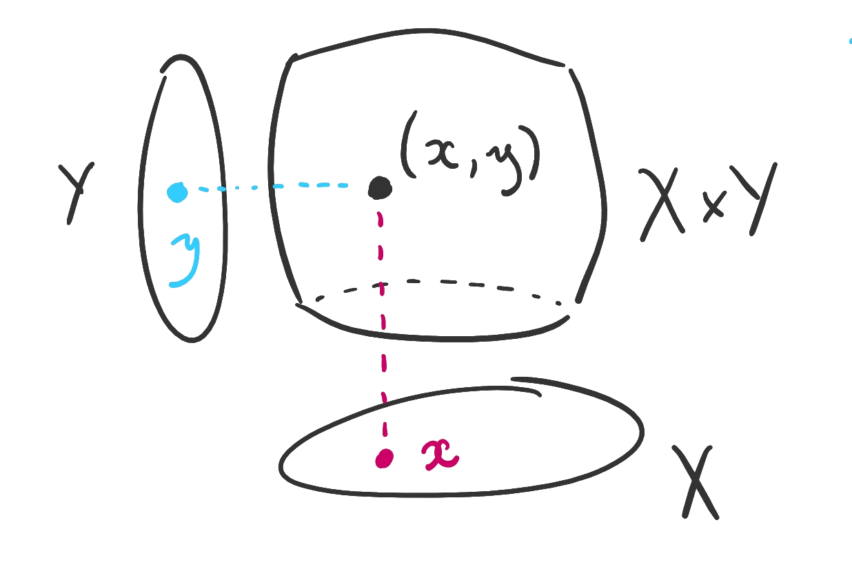
Figure. A visualization of the product of two sets.
Examples. You are likely familiar with , the Cartesian plane from algebra and calculus. The elements of this (infinite) set are ordered pairs where both and are real numbers.
To make a discrete example, put and . Then
As an exercise, calculate yourself. The pair is an element.
Theorem 1.3.7. If and are finite sets, then .
Proof. The elements of may be tabulated into a rectangle, where each row corresponds to an element of and each column corresponds to an element of . There are rows and columns and therefore elements in the table.
1.4 Operations involving more than two sets
Note: While this section is cool, we will not make use of its content very often in this course. You may choose to skip this section for now and return to it after Chapter 8, when you are more comfortable with the material.
There is one last thing to say about sets (for now, anyway). There is no reason to limit ourselves to two sets in union, intersection, and product. If we have a family of sets , we may take -ary unions, intersections, and products.
The -ary union is the set of elements that are in at least one of the sets .
The -ary intersection is the set of elements that are in all of the sets .
The -ary product is the set of ordered -tuples , where the element is a member of the set .
Suppose instead the family is infinite. We will, exactly once in this book, need to take an infinite union. The infinite union is the set of all elements that are in at least one of the . (Notice that the definition hasn’t changed – just the number of sets!) Likewise the infinite intersection is the set of elements in all the .
Takeaways
- A set is a collection of objects. Given a mathematical object, there is almost definitely a way to define that object as a set.
- A given set has many subsets, the collection of which forms its power set.
- The cardinality of a finite set is the number of its elements.
- There are many ways to combine and manipulate sets: union, intersection, difference, and product.
2. Propositional logic
Videos:
- Negation, conjunction, and disjunction
- Conditional statements
- Compound statements
- Rules of inference
- Logical equivalence
In mathematics, we spend a lot of time worried about whether a sentence is true or false. This is fine in the case of a simple sentence such as “The number is prime.” (That sentence is true.) But there are much more complicated sentences lurking around, and whole constellations of sentences whose truth depends on one another. (An unsolved problem in mathematics is deciding whether the Riemann hypothesis, a statement about the prime numbers, is true. Most people believe it is, and many results in the literature are true given the hypothesis. The Riemann hypothesis is going to make or break a lot of research.)
So, we are interested in tools that will allow us to judge whether complicated statements are true. Such models of truth are called logic.
2.1 Statements and connectives
Definition 2.1.1. A statement is a sentence that is either true or false.
Examples. “The number is prime” and “It is perfectly legal to jaywalk” are statements. Non-statements include questions (“Is it raining?”), commands (“Do your homework”), and opinions (“Mint chocolate chip ice cream is the superior flavor”). It is important to note, not necessarily for mathematical purposes, that opinions are statements of pure taste. Claims whose truth values exist but are unknown are beliefs.
Atomic propositional statements of the type discussed in this chapter are flatly always true or false. You may think of them in the same way you think of constant functions in algebra. They are denoted with lowercase letters , , , etc. If the only statements were atomic, logic would be boring. Fortunately, we can combine statements with connectives. In the next chapter, we will look at predicate statements whose truth values depend on an input. Likewise, these may be thought of as the non-constant functions.
Compound statements arise from combining atomic statements with connectives. They are denoted using Greek letters like (“phi”), (“psi”), and (“gamma”). The truth of a compound statement depends on the connectives involved and the truth values of the constituent statements. A tool for determining the truth of a compound statement is called a truth table.
In a truth table for the compound statement , the left side of the table is the atomic statements involved in and the right side of the table is itself. Each row gives a possible combination of truth values for the atomic statements, and the corresponding truth value for . At this point, it is easier to start introducing connectives and seeing some truth tables.
Definition 2.1.2. Let be a statement. Its negation is the statement , the statement that is true exactly when is false and vice-versa.
The statement is typically read "not " or “it is not the case that is true.” If we have an English rendering of , we try to write in a natural-sounding way that also conveys its logical structure.
Example. Suppose represents the statement “It is raining.” Then, stands for “It is not raining.”
Below is the truth table for .
As you can see, on the left are columns corresponding to the atomic statements involved in (just ), and each row is a possible combination of truth values for these statements. Here is a quick, useful theorem without proof:
Theorem 2.1.3. If the compound statement involves different atomic statements, then its truth table has rows.
Look familiar? We will prove this theorem when we prove the related theorem about power sets later on.
Negation is called a unary connective because it only involves one statement. Our remaining connectives are all binary connectives, as they combine two statements.
Definition 2.1.4. Let and be statements. Their conjunction is the statement , which is true only when and are both true.
The symbol in the conjunction is called a “wedge,” and is read " and ." This definition is meant to be analogous to our English understanding of the word “and.” The statements and are called conjuncts.
Example. Letting be “It is raining” and be “I brought an umbrella,” the statement is “It is raining and I brought an umbrella.” The statement is true only if it is currently raining and the speaker brought an umbrella. If it is not raining, or if the speaker did not bring their umbrella, the conjunction is false.
Here is the truth table for :
Notice that this table is organized intentionally, not haphazardly. The rows are divided into halves, where is true in one half and then false in the other half. The rows where is true are further subdivided into half where is true and half where is false. If there were a third letter, we would subdivide the rows again, and so on. This method of organizing the truth table allows us to ensure we did not forget a row. Our leftmost atomic letter column will always be half true followed by half false, and the rightmost atomic letter column will always alternate between true and false.
Definition 2.1.5. Let and be statements. Their disjunction is the statement , which is true if at least one of or is true.
The symbol in the conjunction is called a “vee” and is read " or ." This definition is meant to be analogous to our English understanding of the word “or.” The statements and are called disjuncts. (Did you notice that I was able to copy and paste from an above paragraph? Conjunction and disjunction share a very similar structure.)
Example. Letting be “It is raining” and be “I brought an umbrella,” the statement is “It is raining or I brought an umbrella.” This time, the speaker only needs to meet one of their conditions. They are telling the truth as long as it is raining or they brought an umbrella, or even if both statements are true.
The truth table for follows.
Of great importance to computer science and electrical engineering, but not so much in mathematics (so it will not appear again in this book), is the exclusive disjunction (or “exclusive-or”). It is a modified disjunction where exactly one of the disjuncts must be true.
Definition 2.1.6. If and are statements, their exclusive disjunction is the statement , which is true if and only if exactly one of and is true.
The statement is read " exclusive-or ."
Example. The statement “You can have the soup or the salad” is likely meant as an exclusive disjunction.
In mathematics, disjunctions are generally considered inclusive unless stated otherwise. (An example for us all to follow!)
Our next connective is probably the most important, as it conveys the idea of one statement implying another. As we discussed earlier in the chapter, mathematics is nothing but such statements. It is also the only connective that is not relatively easy to understand given its English interpretation. So we will begin with the truth table, and think carefully about each row.
Definition 2.1.7. If and are statements, the conditional statement is true if can never be true while is false.
There are many ways to read , including “if , then ,” " implies “, and " is sufficient for .” The statement before the arrow is the antecedent and the following statement is the consequent. Here is the conditional’s truth table.
That is true in the bottom two rows may surprise you. So, let’s consider each row separately.
Example. Let be “You clean your room” and be “I will pay you $10,” so that is “If you clean your room, then I will pay you $10.”
In the case that both and are true, the speaker has told the truth. You cleaned, and you were paid. All is well.
In the case that is true but is false, the speaker has lied. You cleaned the room, but you did not earn your money.
What if is false? Well, then the speaker did not lie. The speaker said that if you clean your room you will be paid. If the room isn’t cleaned, then cannot be falsified, no matter where is true or false.
If that explanation is not sufficient for you, reread the definition of the conditional: being true means that cannot be true without . If you are unsatisfied by the English connection, then consider to be a purely formal object whose definition is the above truth table.
Definition 2.1.8. If and are statements, the biconditional statement is true if and are both true, or both false.
The statement may be read as " if and only if , " is necessary and sufficient for ," or " is equivalent to ." Here is the truth table.
Example. Let be “You clean your room” and be “I will pay you $10,” so that is “I will give you $10 if and only if you clean your room.” (The statements were reordered for readability. We will see later in the chapter that this is the same statement, but this wouldn’t work for .) This time, the clean room and the $10 paycheck are in total correspondence; one doesn’t happen without the other.
2.2 Connecting connectives
We are not required to use one connective at a time, of course. Most statements involve two or more connectives being combined at once. If and are statements, then so are: , , , , and . This fact allows us to combine as many connectives and statements as we like.
How should we read the statement ? Should it be read "; also, if then "? Or, “If and , then ?” Just like with arithmetic, there are conventions defining which connective to apply first: negation, then conjunction/disjunction, then implication, then bi-implication. So, "If and , then " is correct. However, to eliminate confusion in this book we will always use parentheses to make our statements clear. Therefore, we would write this statement as .
Remember that a statement involving letters will have rows in its truth table. The column for the left-most statement letter should be true for half the rows then false for half the rows, and you should continue dividing the rows in half so that the right-most statement letter’s column is alternating between true and false.
Finally, it is a good idea to break a statement into small “chunks” and make a column for each “chunk” separately. Observe the following example.
Example. Write down the truth table for the statement . When is this statement false?
Since the statement has letters, there will be rows to the truth table. Let’s go through the first row very slowly, where all four atomic statements are true. Then is true and is false. Since is true and is false, that means is false. Finally, because its antecedent is true and its consequent is false, the compound statement would be false.
Here is the full truth table. Be sure you understand how each row is calculated.
There are tricks to calculate truth tables more efficiently. However, it wouldn’t do you any good to read them; they must come with practice.
2.3 Inference and equivalence
Mathematics is all about relationships. If the statement is always true, then it tells us that whenever is true then must be as well. If the statement is always true, then it tells us that from the point of view of logic and are actually the same statement. That is, it is never possible for them to have different truth values.
Definition 2.3.1. A tautology is a statement that is always true, denoted .
Definition 2.3.2. A contradiction is a statement that is always false, denoted .
Definition 2.3.3. A rule of inference is a tautological conditional statement. If is a rule of inference, then we say implies and write .
Remember that a conditional statement does not say that its antecedent and consequent are both true. It says that if its antecedent is true, its consequent must also be true.
There are many rules of inference, but we will explore two.
Definition 2.3.4. Modus ponens is the statement that says we may infer from and . Symbolically:
Example. Consider the conditional statement “If you clean your room, then I will give you $10.” If the speaker is trustworthy, and we clean our room, then we may conclude we will be receiving $10.
Another example: “If a function is differentiable, then it is continuous.” (You may know the meanings of these words, but it is not important.) If this statement is true, and the function is differentiable, then without any further work we know that is continuous.
Theorem 2.3.5. Modus ponens is a rule of inference.
Notice that in the definition no claim is made that modus ponens is always true. That is up to us.
Since we know how to use truth tables, we may construct one to show that is always true. Before reading the table below, try to make your own!
Proof. The above table shows that is true no matter the truth of and .
Definition 2.3.6. In the context of conditional statements, transitivity is the rule that if implies and implies , then implies . Or,
The wording of the definition above should you make you suspicious that this is not the only time we will see transitivity. In fact, you may have seen it before…
Example. If you give a mouse a cookie, then he will ask for a glass of milk. If he asks for a glass of milk, then he will also ask for a straw. Therefore, if you give a mouse of cookie then he will ask for a straw.
Theorem 2.3.7. Transitivity is a rule of inference.
We could simply write down another truth table and call it a day. In fact, go ahead and make sure you can prove transitivity with a truth table. Once you’re done, we’ll try something slicker to prove transitivity.
Proof. Suppose that and are true statements, and that moreover is true. By modus ponens, must also be true. Then, is true, by a second application of modus ponens. Therefore, if is true, must be also; this is the definition of .
Pretty cool, right? We can cite proven theorems to prove a new one.
Does it work the other way? In other words: if I know that , does that mean ? Regrettably, no: consider the case there and are true but is false.
Some rules of inference do work both ways. These are called equivalences.
Definition 2.3.8. If is a tautology, then it is an equivalence and and are equivalent statements. We write .
Equivalent statements are not the same statements, but they are close enough from the point of view of logic. Equivalent statements are interchangeable, and may be freely substituted with one another.
We will quickly run through many equivalences before slowing down to prove a few.
Algebraic properties of conjunction, disjunction, and negation
Our first batch of statements should look familiar to you; these are the ways that statements “act like” numbers. As you read each one, try to justify to yourself why it might be true. If you aren’t sure of one, make a truth table.
| Equivalence | Name |
|---|---|
| Double negation | |
| Commutative of conjunction | |
| Commutative of disjunction | |
| Associativity of conjunction | |
| Associativity of disjunction | |
| Conjunctive identity | |
| Disjunctive identity | |
| Conjunctive absorption | |
| Disjunctive absorption | |
| Conjunctive cancellation | |
| Disjunctive cancellation |
Distributive properties
In our numbers, multiplication distributes over addition. This is one fact that is likely implemented twice in your head, once for a number: and once for “the negative” (truly the number ): However, these rules are one and the same; the distributive law. Likewise, we will have distributive laws for negation, conjunction, and disjunction.
| Equivalence | Name |
|---|---|
| DeMorgan’s law | |
| DeMorgan’s law | |
| Conjunction over disjunction | |
| Disjunction over conjunction |
DeMorgan’s law is one of the most important facts in basic logic. In fact, we will see it three times before we are through. In English, DeMorgan’s law says that the negation of a conjunction is a disjunction and vice-versa.
To show that and are equivalent, we can show that the biconditional statement is a tautology. Thinking about the definition of the biconditional gives us another way: we can show that the truth tables of and are the same; in other words, that both statements are always true and false for the same values of and .
Proof (of DeMorgan’s law for conjunction). Let and be statements. The statements and are equivalent, as shown by the below truth table.
Therefore, .
You’ll notice a few columns are skipped in the above truth table. After a few tables, it is more convenient to skip “easy” columns. For example, we know that is true only when and are both true, and false everywhere else. Therefore, we can “flip” that column to quickly get the column for .
As an exercise, prove DeMorgan’s other law.
Properties of the conditional
Finally, we come to the properties of conditional (and biconditional) statements. These do not have “obvious” numerical counterparts, but are useful all the same.
| Equivalence | Name |
|---|---|
| Material implication | |
| False conditional | |
| Contraposition | |
| Mutual implication |
Material implication is the surprising result that the conditional is just a jumped-up disjunction! In fact, DeMorgan’s law, material implication, and mutual implication together prove that all of the connectives we’ve studied can be implemented with just two: negation and one other. However, this would make things difficult to read, so we allow the redundancy of five connectives.
Let’s prove material implication with a truth table, and then we will prove contraposition with another method.
Proof (of material implication). Let and be statements and observe that the truth tables for and are the same:
Therefore, .
There is another way to think about material implication. The statement means that never happens without . Another way to say this is that happens, or else did not; so, .
Before we prove contraposition by the other method, we must justify said method with a theorem.
Theorem 2.3.9. Statements and are equivalent if and only if and are both rules of inference.
The phrase “if and only if” in a mathematical statement means that the statement “works both ways.” In this case, means and are both rules of inference; and conversely, and both being rules of inference means . It means that “” and “” and are both rules of inference" are equivalent statements. Fortunately, we already have a rule that justifies this equivalence.
Proof (of Theorem 2.3.9). Mutual implication says that .
It’s that easy. Whenever we have a conditional statement and its converse (the order reversed), we have the biconditional; likewise, we may trade in a biconditional for two converse conditional statements.
Now we will prove contraposition by showing that implies , and vice-versa. Before you read the below proof, write down these rules: material implication, double negation, and commutativity of disjunction.
Proof (of contraposition). Suppose and are statements and that is true. By material implication, is true. Commutativity says this is the same as . So, we may apply material implication backwards, negating this time, to get ; therefore, implies .
Conversely, suppose is true. Then material implication (and double negation) gives . We may commute the disjunction and apply material implication again, negating , to get .
By mutual implication, .
Takeaways
- Statements may be modified and combined in (mainly) five ways: negation, conjunction, disjunction, implication (the conditional), and bi-implication (the biconditional).
- A truth table allows us to see when a compound statement will be true or false.
- If one statement always implies another, that implication is a rule of inference.
- If two statements are always true or always false together, they are equivalent.
- Rules of inference and equivalences may be justified with truth tables or algebraically.
3. Predicate logic
Videos:
- Predicates
- Introduction to quantifiers
- Quantifiers, continued
- Inference and equivalence with quantifiers
3.1 Predicates
Basic propositional logic as you learned it in the preceding chapter is powerful enough to give us the tools we will need to prove many theorems. However, it is deficient in one key area. Consider the following example.
Example. If Hypatia is a woman and all women are mortal, then Hypatia is mortal.
We can all agree that this statement is a tautology; that is, if it is true that Hypatia is a woman (she was; she was a Greek mathematician contemporary with Diophantus) and if it is true that all women are mortal (as far as we know this is the case) then it must follow that Hypatia is mortal (she was murdered in 415).
So the statement is a tautology. If so, the truth table would confirm it. Let symbolize the statement, where stands for the statement that Hypatia is mortal.
Oh no! Our second row gives that the statement is false when is false but and are true. What gives?
Well, consider the statement “If pigs fly and the Pope turns into a bear, then Bob will earn an A on the exam.” Now it is not so clear that this is a tautology, because pigs, the Pope, and Bob’s grade presumably have nothing to do with one another.
But Hypatia and the mortality of women do. What we will need is the ability to signify that two statements are related, whether in subject (e.g. Hypatia) or predicate (e.g. mortality). This is where predicate logic comes in to help.
Definition 3.1.1. A predicate is a function that takes one or more subjects (members of some domain ) and assigns to them all either true or false .
Predicates are typically denoted with capital letters like , , and . Subjects that are known are given lowercase letters like , , and , unless there is something more reasonable to pick like for Hypatia. Subjects whose values are unknown or arbitrary are denoted with lowercase , , , etc.
The definition of predicate above is much more complicated than it needs to be; this is so that we can take the central idea (a function) and continue using it throughout the book. You know a function: an assigment that gives every input exactly one output . We write to signify that is a function whose inputs are elements of the set and whose outputs are elements of the set .
So, in the above definition, the predicate is a function that takes a subject, a member of the set , and assigns it exactly one truth value.
(Take note that propositions, which you studied in the last chapter, may be regarded as constant predicates – functions whose value is the same regardless of the input, like .)
Examples. Letting be the predicate " is a woman" on the domain of humans and stand for Hypatia, is the statement “Hypatia is a woman.” Since this statement is true, the function assigns to .
Let be the predicate “” on the domain and let be the predicate " orbits " on the domain of celestial objects in the sky. The statement is true, but is false. If stands for the earth and for the sun, then is false but is true.
A predicate, once evaluated to a subject, is a statement. Therefore, these statements may be combined into compound statements using the logical connectives we have just studied.
Examples. As before let be the predicate “” on the domain and let be the predicate " orbits " on the domain of celestial objects in the sky, where stands for the earth and for the sun.
The statements , , and are true.
The statements and ae false.
3.2 Quantifiers
This is all well and good, you think, but what about the statement “All women are mortal”? How can we make “all women” the subject of a statement?
Quantifiers allow us to say that a predicate is true for all, or for at least one undetermined, object in its domain.
Definition 3.2.1 Let be a predicate. The universal statement says that is true for all in its domain. The symbol (“for all”) is called the universal quantifier.
Example. The domain is very important. If is the predicate " takes discrete math" then – “Everyone takes discrete math” – is true on the domain of computer science students at Coastal Carolina, but not, say, on the domain of all people in South Carolina.
Definition 3.2.2 Let be a predicate. The existential statement says that is true for at least one in its domain. The symbol (“there exists”) is called the existential quantifier.
Example. Again let be the predicate " takes discrete math". The existential statement says “Someone takes discrete math.” This is now true for people in South Carolina – pick a student at Coastal, or Clemson, or USC – but not true on the domain of dogs. Wouldn’t that be cute, though?
The statement operated on by a quantifier is called its scope. Without parentheses, a quantifier is considered to apply only to the statement it is next to and no others.
Examples. Let be the predicate " takes discrete math" and be the predicate " is a math major".
- The statement means “There is someone who is taking discrete math and is a math major.” Both and apply to the same .
- The statement says “Someone is taking discrete math and someone is a math major.” The subjects of and are possibly different.
- The expression is not a statement at all, because is not a statement. It needs either a quantifier, or for to refer to a specific, known member of the domain.
There are two important quantified statements: “All 's are 's” and "Some is a ". These statements are all over the place in mathematics. We like to characterize mathematical objects by saying all objects of one type also belong to another; or, by saying we can find an object of one type that is another type.
In “All 's are 's”, the word “all” suggests that the universal quantifier is appropriate. What connective should be used to combine the predicates? Observe that the statement says that every is both a and a . This isn’t what we mean to say; we mean to say if something is a then it will also be a . So, the correct rendering of “All 's are 's” is .
For the statement “Some 's are 's”, we mean to say that there is an object that is at once a and a . Therefore, this time the conjunction is appropriate: we write .
| Statement | Implementation |
|---|---|
| “All 's are 's” | |
| “Some 's are 's” |
Finally, what is to be done with statements with two or more subjects? The ordering of the quantifiers matters. Here are the four possible combinations of universal and existential quantifiers for two subjects, as well as a diagram corresponding to each.
Examples. Let be the predicate " and are classmates" over the domain of students at some school. Note that, in this case, the order of the subjects does not affect the truth of the statement.
The statement means “There are two students who are classmates.” In other words, there is at least one student who is paired with at least one other student. Some writers say instead, but when the quantifiers are the same we will “collapse” the notation.
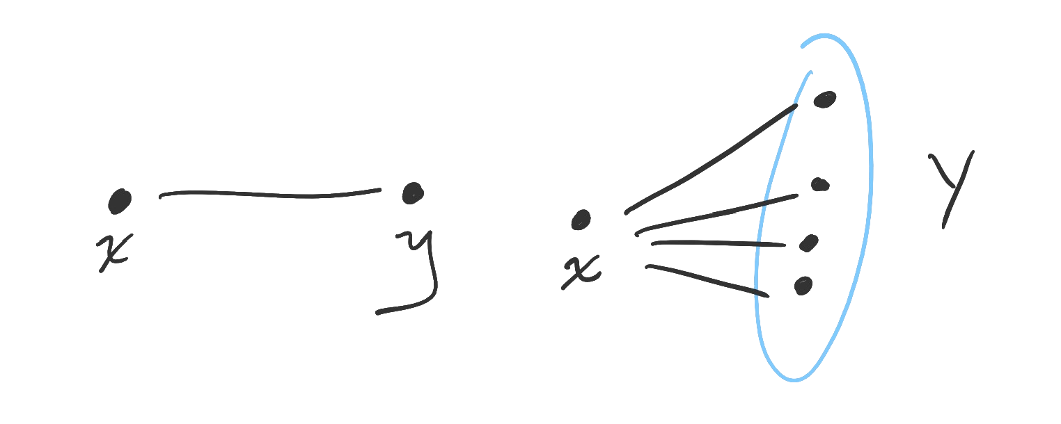
Figure. On the left, one object is paired with one object (existential-existential). On the right, one object is paired with many objects (existential-universal).
The statement means “There is a student who is classmates with every student.” We have one student who (somehow!) is classmates with the entire student body.
The statement means “Every student has a classmate.” Notice that their classmate need not be the same person. If we quantify universally first, then each existential object may be different. In the preceding example, we quantified existentially first, so that one person was classmates with everybody.
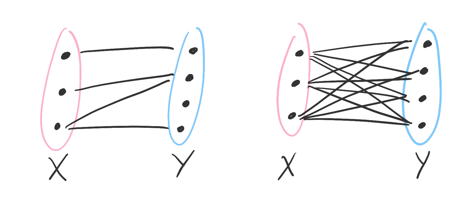
Figure. On the left, many objects are each paired with an object (universal-existential). On the right, many objects are paired with many objects (universal-universal).
The statement means “Every student is classmates with every other student.” Every object in our domain is paired up with every other object in the domain, including themselves! (Don’t think too hard about that for this example.)
3.3 Inferences and equivalences for quantifiers
Quantifiers evaluated on a predicate are statements, since they are functions to . Therefore, some quantified statements imply others, and some pairs imply each other. In this section we will learn a few important rules for quantifiers, before finally proving that our opening statement about Hypatia is indeed a tautology.
Theorem 3.3.1 (DeMorgan’s laws) Let be a predicate. Then and .
Does that name look familiar? Here is our second application of DeMorgan’s laws. (The third will appear in the exercises.) You will see how they are used in the proof.
Proof. Consider the universal statement on the domain . We may rewrite
and
Therefore,
Using DeMorgan’s law,
which is the same as the statement .
That may be proven in the same way.
The idea is that a universal statement is a “big conjunction” and an existential statement is a “big disjunction.” The proof follows from the DeMorgan’s laws you learned in the preceding chapter .
The next two theorems deal with how universal and existential statements may imply one another.
Theorem 3.3.2 (Universal instantiation) If is a member of the domain of the predicate , then .
Proof. If is true for every member of its domain and is a member of said domain, must be true for .
Theorem 3.3.3 (Existential generalization) If is a member of the domain of the predicate , then .
Proof. Let be in the domain of . If is true, then is true for some member of its domain.
There are two comments to make about these two theorems. First, universal generalization and existential instantiation are not valid:
Examples. “I was able to easily pay off my college loans, therefore everyone can” is an example of invalid universal generalization.
“Someone in this room killed the wealthy magnate, so it must have been you!” is an example of invalid existential instantiation.
Finally, transitivity gives us that a universal statement implies an existential one: .
We are ready to prove our tautology is, in fact, a tautology. Remember that the statement was “If Hypatia is a woman and all women are mortal, then Hypatia is mortal.”
We have seen that “Hypatia is a woman” may be rendered as for the predicate being " is a woman" and being Hypatia. Likewise, “Hypatia is mortal” could be rendered where is " is mortal". Finally, the statement “All women are mortal” would be .
Theorem 3.3.4 The statement is a tautology.
We have changed our labeling to the more standard , , and to emphasize that this statement is always true no matter what we are talking about.
Proof. Suppose that for some predicate and some in the domain of that is true, and that for some predicate the statement is true.
By universal instantiation, means that is true.
By modus ponens on and , we know must be true.
Therefore, is always true.
Takeaways
- If we need to communicate that two statements talk about the same thing, propositional logic won’t cut it: we need predicates.
- A predicate is a function that takes an input and returns true or false. The predicate itself isn’t a statement, but it is once it’s evaluated on a subject.
- A quantifier yields a statement that a predicate is true for some, or all, objects in its domain.
- "Every – is a – " is a universal conditional statement. "Some – is a – " is an existential conjunction.
- A universal statement implies a specific one, which implies an existential statement.
- The negation of a universal statement is an existential statement and vice-versa.
Proofs
Review:
- Chapter 2: Inferences and equivalences for conditional and biconditional statements
- Chapter 3: Inferences and equivalences for quantifiers
Videos:
Now we have things to talk about – sets and their elements – and ways of talking about those things – propositional and predicate logic. This opens the door to the true game of mathematics: proof.
Mathematics stands apart from the natural sciences because its facts must be proven. Whereas theories in the natural sciences can only be supported by evidence, mathematical facts can be shown to be indisputably true based on the agreed definitions and axioms.
For example, once you have agreed upon the definitions of “integer,” “even,” and the rules of arithmetic, the statement “An even integer plus an even integer is an even integer” is without doubt. In fact, you will prove this statement yourself in the exercises to this chapter.
Now, this introduction is not meant to imply that mathematical epistemology (the study of knowledge) is without its issues. For example: What definitions and axioms are good ones? (“Is there such a thing as a real number?” can entertain you for a while.) What sorts of people decide which mathematical research is worth doing, and who decides which proofs are convincing? Are all published mathematical proofs correct? (They aren’t.) What is the role of computers in mathematical proof?
Fortunately for us, we don’t have to worry about these questions. (Unless we want to. They’re quite interesting.) In this chapter we will simply learn what a mathematical proof is, learn some basic facts about the integers, and practice writing direct and indirect proofs about mathematical facts that are not particularly in dispute.
4.1 Direct proofs
What is a proof? In this book we will adopt Cathy O’Neil’s position that a proof is a social action between speaker/writer and listener/reader that convinces the second party that a statement is true.
Several proofs have been written in this book so far. Many begin with an italicized Proof. and end in a little , as a way to set them off from definitions, theorems, comments, and examples. Hopefully they have all been convincing to you. (DW: If not, my e-mail address is somewhere on this webpage.)
As you practice writing your own proofs, take for an audience someone else in your position: a new student of discrete mathematics. Imagine the reader knows slightly less than you do. A good proof gently guides the reader along, making them feel smart when they anticipate a move.
It is also this book’s position that talking about proofs is nearly useless. They must be read and practiced. With that in mind, let’s get to writing some proofs about integers.
We will take for granted that sums, differences, products, and powers of integers are still integers. (Depending on how the set of integers is defined, these qualities may be “baked in” to the definition.) Every other fact will either be stated as a definition or a theorem, and proven in the latter case.
Definition 4.1.1. An integer is even if there exists an integer such that .
Definition 4.1.2. An integer is odd if there exists an integer such that .
For examples, , and .
Theorem 4.1.3. If an integer is odd, so is .
This statement may be obvious to you. If so, great; but we are trying to learn about the writing, so it is best to keep the mathematics simple. (It will only get a little more challenging by the end of the chapter.) To prove this statement, we must start with an arbitrary odd integer and prove that its square is odd. The integer in question must be arbitrary: if we prove the statement for 3, then we must justify 5, 7, 9, and so on.
Proof. Let be an odd integer.
The first step in the proof is to assume any of the theorem’s hypotheses. The theorem says that if we have an odd integer, its square we will be odd; so, we are entitled to assume an odd integer. However, there is nothing more we may assume. Fortunately, we know what it means for an integer to be odd.
That means there exists an integer such that .
A great second step is to “unpack” any definitions involved in the assumptions made. We assumed was odd. Well, what does that mean? However, now we are “out of road.” Let’s turn our attention to the object we mean to say something about; .
Therefore, which is an odd number by definition.
Remember: sums, powers and products of integers are integers – this is the only thing we take for granted, other than, y’know, arithmetic – and so is an integer, call it . Then is odd. The final step – obviously rendering the result in the explicit form of an odd number – is a good one to take because we assume our reader to be as new at this as we are. They likely recognize is odd, but we take the additional step to ensure maximum clarity.
Thus, if is an odd integer so is its square.
Definition 4.1.4. Let be a nonzero integer and let be an integer. We say divides or that is divisible by if there exists an integer such that . We write when this is the case.
Theorem 4.1.5. Divisibility has the following three properties:
- For all integers , . (reflexiveness)
- For all positive integers and , if and then . (antisymmetry)
- For all integers , , and , if and then . (transitivity)
(These three properties together define something called a partial order, which is studied in the last chapter. Foreshadowing!)
You will prove two of these properties for yourself in the exercises. Here is a demonstration of the proof of the second property.
Proof. Suppose that and are positive integers where and .
As before, we are assuming only what is assumed in the statement of the theorem: that and are positive divide one another. By the way: why did we have to say they are positive?
That means that there exist integers and such that and .
The second step is usually to apply relevant definitions.
Combining these two statements, we have . Since is not zero, we see . Because and must be integers by definition, the only way that is for .
If we didn’t have the restriction that and were integers, then . However, this is only possible for integers when both numbers are one.
Therefore, if and are positive integers that divide one another, then .
In the next section we will explore indirect proofs and, from there, bidirectional proofs. You are highly recommended to try some exercises before moving on.
4.2 Indirect and bidirectional proofs
Consider the following theorem.
Theorem 4.2.1 If is an integer such that is odd, then is odd.
This theorem may seem the same as Theorem 4.1.3, but note carefully that it is not: it is the converse to the previous theorem’s .
Let’s try to imagine a direct proof of this theorem. Since is odd, there exists an integer such that . And then, seeking to prove a fact about , we take the positive square root of each side: . And…ew. Have we even proven anything about square roots? (We haven’t, and we won’t.)
We shall, instead, employ some sleight of hand. Recall from Chapter 2 that a conditional statement is equivalent to its contrapositive .
Proof (of Theorem 4.2.1). Suppose that is even. Then there exists an integer such that . In that case, which is even. Therefore for to be odd, must also be odd.
Another equivalence from Chapter 2 was that and combine to create . That is, we can prove an “if and only if” statement by proving both the “forward” and “backward” directions (which is which is a matter of perception). Therefore, in this chapter we have proven the following statement:
Theorem 4.2.2 An integer is odd if and only if is.
Remember that an “if and only if” statement is true if the component statements are both true or both false. So, this theorem also tells us that an integer is even if and only if its square is.
Theorem 4.2.3 Let be an integer. The integer is odd if and only if is even.
Proof. Let be an integer. First, suppose is odd. That means that there exists an integer where . So, which may be written as which is even. Therefore if is odd then is even.
Conversely, suppose is even. That means that for some integer . In that case, which is which is odd. Therefore for to be even, must be odd.
So, is odd if and only if is even.
4.3 Counterexamples
When proving a universal statement on a domain, it never suffices to just do examples (unless you do every example, which is usually not feasible or possible). However, remember from Chapter 3 that the negation of a universal statement is an existential one. You can prove that "every is a " is false by finding just one that isn’t a .
Examples. The statement “all prime numbers are odd” is false because is prime and even.
The statement “all odd numbers are prime” is false because is odd and not prime.
Takeaways
- A proof is a social action between speaker and listener. Keep your audience in mind as you write - try to make them feel smart! If you are taking a class, your proofs should be written for your classmates.
- If you are trying to prove that a statement is true for every object of a particular type, it is never appropriate to just do a couple of examples.
- In a direct proof of , you should start by assuming any hypotheses and unpacking the relevant definitions before arriving at the conclusion via valid reasoning.
- Sometimes it is hard to prove directly, in which case maybe you should try proving the contrapositive .
- You can prove by proving and .
- You have to practice proof writing a lot. (DW: I wasn’t a good proof writer until the end of graduate school, and one may argue I am still not a good proof writer.)
5. Recursion and integer representation
Videos:
One of the most important ideas in discrete mathematics is that of recursion, which we will explore in one way or another for many of the remaining chapters in the course. In this chapter, we will explore it through the idea of integer representation; representing integers in bases other than the common base 10. Bases you are likely to encounter in computer science contexts are base 2 (binary), base 8 (octal), and base 16 (hexadecimal). We will learn how to represent an integer in binary using a recursive algorithm, and then we will cheat our way into octal and hexadecimal.
5.1 Recursion
Recursion is when an algorithm, object, or calculation is constructed recursively.
Just kidding. Reread this joke after the chapter and it’ll make more sense.
Recursion means that an algorithm, object, or calculation is written, defined, or performed by making reference to itself. It is something more easily understood by example, and there will be plenty as we proceed. For now, consider the following example.
Definition 5.1.1 Let be a positive integer. Then (" factorial") is the product of all positive integers at most : Furthermore, we define .
Anyone questioning the usefulness of will have their questions answered in excruciating detail over the course of Chapters 9-13. If the reader has had calculus, then they may recognize as the denominator of the terms in the Taylor expansion of the function ; it is good for “absorbing” constants created by taking derivatives. However, we are not interested in any of its uses right now.
Example. Here are the values of a few factorials: , , , , , and .
You may have already noticed the recursion at work. Take for instance . We see the value of lurking here: .
In fact, for all positive , we can make the alternative (usually more useful) definition . This is the recursive defintion of the factorial, because we are defining the factorial in terms of the factorial.
Why is this okay? Well, we’re really collapsing a lot of work into two lines: it may make more sense to break it down one step at a time. First, define . This definition will make sense in a later chapter, but remember that mathematical definitions don’t necessarily need to “make sense.”
Next, define . This definition is valid, because the number , the operation , and the number have all been defined. And when we go to define , we have already defined all of these objects as well. And so on. Therefore, the following definition is a valid one.
Definition 5.1.2 Let be a natural number. Then is equal to 1 when , and otherwise.
5.2 Binary numbers
Now that we know how recursion works (or at least have more of an inkling than we did upon starting the chapter), we will see another example of it in the calculation of the binary representation of a number.
When we speak of the number one thousand five hundred eight or , we are implicitly talking about the composition of the number in terms of powers of 10: remembering that for all nonzero .
African and Asian mathematicians were writing in base-10, or decimal notation, as early as 3,000 BCE. Presumably the prevalence of decimal notation throughout human history is due to the fact that most of us have ten fingers and ten toes, making the base convenient. However, computers only have two fingers and two toes.
That last line is a joke, but here’s the idea: Computers read information by way of electrical signals, which are either on or off. So the simplest way for a computer to process information is in terms of two states. Here is a higher-level example: suppose you are writing some code. Is it easier to have a single if-then statement (two possible states), or nine (ten possible states)? This is why base-2, or binary numbers, are so prevalent in computer science.
The first step to becoming adept with binary numbers is to know many powers of . Fortunately, powers of are easy to calculate: simply multiply the last value by to get the next one. (This is a recursive definition for !)
Algorithm 5.2.1 Let be a natural number. To write the -digit binary expansion of :
- If , its binary expansion is .
- If , its binary expansion is .
- If , find the highest number such that . This is the number of binary digits of . Then, the binary expansion of is . The remaining digits , , , , are the digits of binary expansion of , or if the binary expansion of does not contain that digit.
This is perhaps a little intimidating at first glance, so let’s press on with an example.
Example. Let’s calculate the binary expansion of . Our target is neither nor , so we must find the highest power of that is no more than . This number is . Therefore, our binary number will have eleven digits, and right now it looks like
To find the values of the remaining digits , , etc., let’s find the binary expansion of the remainder .
Here’s the recursion, by the way: to find the binary expansion of , we must find the binary expansion of a smaller number.
We repeat the process. The highest power of that divides is . So, the binary expansion of is the nine-digit number Be aware that it is okay to reuse the names for the unknown digits, because the algorithm says they are the same for both numbers.
Next, we find the second remainder The highest power of 2 dividing 228 is Continue the example and see for yourself that the binary expansion of is . (Your remainders after will be , , , and .)
Now, the binary expansion of is and the binary expansion of is
The algorithm tells us what to do with our missing : since it does not appear in the expansions of any of our remainders, it is 0. Therefore,
This examples was made much more tedious than it needed to be so that the recursive steps were laid bare. In practice, you will simply continue subtracting off powers of until none of the target number remains, writing a if you subtracted a particular power of and a if you didn’t. Since we had to subtract , , , , , and , we write a for the eleventh, ninth, eighth, seventh, sixth, and third digits, and a everywhere else.
You have no doubt noticed that our binary numbers are all enclosed in the notation . This is to signify that the , for example, is referring to the number five and not the number one hundred one.
5.3 Octal and hexadecimal numbers
The word octal refers to the base-8 system and hexadecimal refers to the base-16 system. These two bases are useful abbreviations of binary numbers: octal numbers are used to modify permissions on Unix systems, and hexadecimal numbers are used to encode colors in graphic design.
We say “abbreviation” because of the following algorithm.
Algorithm 5.3.1 Suppose is an integer with a base representation and we desire to know its base representation, for some integer . Then we may group the digits of in base into groups of and rewrite each group as a digit in base . The resulting string is the binary expansion of in base .
The idea is that it is easy to go from some base to a base that is a power of the original base. Consider the following example.
Example. Write the number in octal and in hexadecimal.
The starting point will be to write in binary. Since its binary expansion is .
To write in octal, we will regroup the binary digits of by threes because . However, there are eight digits. No worries; we will simply add a meaningless as the leftmost digit of the binary expansion. Those groups are: , , and from left to right. In order, those numbers are , , and ; so, is .
Observe that in a base number system, the digits are . Therefore the highest digit we will see in octal is .
However – what about hexadecimal? Its set of digits is larger than our usual base-10 set. It is standard usage to use through to represent through .
| Decimal digit | ||||||
|---|---|---|---|---|---|---|
| Hexadecimal digit |
Since , to write in hexadecimal we will group the digits in its binary expansion by fours this time. Those groups are and , which represent fourteen and twelve respectively. So, .
To summarize our example, here are four different representations of the number .
| System | Decimal | Binary | Octal | Hexadecimal |
|---|---|---|---|---|
Takeaways
- Recursion is when something is defined or implemented in terms of its own definition or implementation. Recursion is incredibly useful both mathematically and programmatically.
- Given a positive integer , its factorial – the product of all positive integers at most – may be recursively expressed as . Meanwhile, .
- Binary numbers are convenient in programming. We may write a binary number by recursively writing a smaller number in binary first.
- We may express a binary number in octal or hexadecimal by grouping its digits by threes or fours.
6. Sequences and sums
Videos:
- Introduction to sequences
- Recurrence relations
- Directly calculating sums
- Indirectly calculating sums
6.1 Sequences
Remember that a set has no order. For example, and are the same set. Often, we care about the order objects are in. Enter the sequence.
Definition 6.1.1 Let and be some set. A sequence is a function . We write instead of . Here, is the index and is the term. We denote the entire sequence as (when the start and endpoints are stated elsewhere or are unimportant), (for an infinite sequence starting with ), or (for a finite sequence starting at and ending at ). A finite sequence is called a word from the alphabet .
Once again we have chosen a more technical, functional definition where we instead could have said “a sequence is a totally ordered list of objects.” It is worth considering the way in which a function can “port structure” from one set to another. If we wanted a totally ordered set it is hard to imagine a better candidate than . The sequence transfers the order structure from into whatever set we like.
Example. Consider the sequence Observing that each term is the square of its index, this sequence may be represented in closed form by writing .
Not every sequence may be so easily identified in closed form.
Example. Consider the sequence You may recognize this sequence as the famous Fibonacci sequence. There is a closed-form expression for , but you are unlikely to see it by visual inspection. However, notice that each term in the sequence is equal to the sum of the preceding two terms: for instance, .
Therefore instead we can represent the Fibonacci sequence recursively with a recurrence relation:
Once a recurrence relation is established, the terms of a sequence may be calculated iteratively or recursively. Each method has its strengths and weaknesses depending on the context; typically, recursive calculations are more difficult but require storing less information.
Example. Consider the sequence where
To calculate iteratively, we simply calculate each term of until we arrive at . So: , and . Then and Thus, .
In the recursive calculation, we will begin with and repeatedly apply the recurrence relation until we have only known values of the sequence: so, and . First, However, we “don’t know” what is, so we repeat the recursion: Now we substitute in the given values: It is important that we arrive at the same value both ways!
6.2 Sums
Given a sequence, a natural course of action is to add its terms together. To avoid writing a bunch of plus signs, we write for the sum of the members of , starting with the -th member and ending with the -th member.
Example. Consider the sum Notice that is being used for the index rather than . That’s okay! The sum’s value is
We can have sums of sums, and sums of sums of sums, etc. Double sums are common in computer science when evaluating the runtimes of doubly-nested for loops.
Example. Consider the sum This sum is rectangular in the sense that the bounds of one sum are not determined by the other, and so we could do this sum in either order: or Either way, the sum’s value is .
For another example, take Because the bounds of the -sum are dependent on the value of , we should iterate over first:
Each of these sums must be done separately. The first sum, of just one term, is equal to . The second sum is , the third is , and the fourth is ; so altogether the sum is .
We will end on two theorems that are important for manipulating sums, the second of which will be very useful later.
Theorem 6.2.1 [Linear property of summation] Let and be sequences and be a constant value. Then, and
Proof. The associative property of addition – – and the distributive property – – guarantee this theorem.
Example. Suppose we know that Then the value of the sum is Notice that both sums must start and end on the same index.
Theorem 6.2.2 [Recursive property of summation] Let be a sequence. Then
Proof. By definition, By the associative property of addition we may rewrite this as either or proving the theorem.
Example. Suppose it is known that and that Then,
Takeaways
- A sequence is a (possibly infinite) ordered collection of objects.
- Terms of a sequences may be defined in closed form, via a formula, or recursively based on prior terms of the sequence.
- Sums may be calculated directly or indirectly, using linearity or recursiveness.
7. Asymptotics
Videos:
Consider the following example of two programs, and , that process some data. The following table provides the number of computations taken by each program to process data points.
| Program | Program | |
|---|---|---|
| 1 | 1 | 58 |
| 10 | 100 | 508 |
| 20 | 400 | 1008 |
| 50 | 2500 | 2508 |
| 60 | 3600 | 3008 |
| 100 | 10,000 | 5008 |
At first, Program looks much better than Program . However, as increases, it becomes clear that is worse at handling large quantities of data than . If and represent sequences of the numbers of steps taken by each program, then and . The way we quantify the relationship between the two sequences is by saying is “big-O” of .
7.1 Growth bounds on sequences
Definition 7.1.1 Let and be terms of sequences. We say is big-O of if there exist a real number and an integer such that for all , We write , even if the equals sign is technically incorrect.
This is another technical definition that can be hard to parse, but the idea is that eventually (after the -th term of the sequence) does not grow faster than . In this way, serves as an upper bound on the growth of .
As we will see again in Chapter 18, there may be many upper bounds. For example in a classroom of twenty-nine students I may say “Here are fewer than thirty students” or “Here are fewer than a million students.” The first statement is obviously more informative. So often you will be asked to find the least upper bound on the growth of ; this is usually a that is the simplest and is itself big-O of all the other options.
Theorem 7.1.2 Any non-negative sequence is big-O of itself.
Proof. Let be a non-negative sequence; that is, for all . Then the statement is satisfied by equality since . If we put , then this statement implies that .
We can form a basic hierarchy of sequences and their big-O relationships. In the below table, a sequence appearing to the left of a sequence means that .
| Slowest | Fastest | ||||||
|---|---|---|---|---|---|---|---|
At the left-most end of the chart, the slowest-growing sequence is . It is slowest-growing because it does not grow at all! In fact, any constant sequence is big-O of any other sequence.
Next is the sequence . In this book, refers to the base-2 logarithm that you might have elsewhere seen written as . Here are a couple of ways to conceptualize this sequence and its relevance to computer science.
- is big-O of the number of digits in the binary expansion of .
- is roughly the number of times a finite sequence of length can be cut in half.
The rest of the functions in the list should be familiar. Notice that all polynomial functions of higher degrees appear between and , and higher-order exponential functions like occur between and .
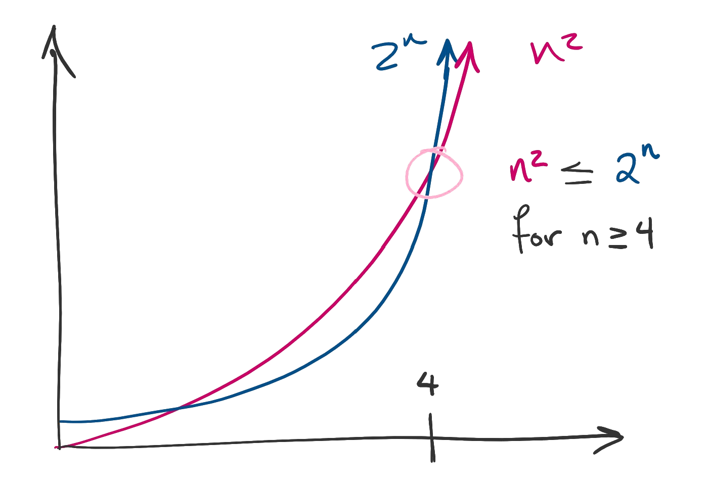
Figure. Two graphs are compared. Since after a point the blue graph is always above the red graph, the function in red is big-O of the function in blue.
Now we know where basic functions fit into the big-O hierarchy, but what about more complicated expressions like ? The following theorem will help.
Theorem 7.1.3 Let and be sequences.
- If is a nonzero constant, then .
- Suppose there exists a sequence such that and . Then, is big-O of as well.
- Suppose there exist sequences and such that and . Then, .
In plain English, this theorem says:
- Constant multiples do not affect growth rate.
- When adding two sequences, the larger absorbs the smaller. In other words, one must only look at the highest-order term of a sum.
- Growth rates are multiplicative; “big-O of the product is the product of the big-O’s,” though that language is very informal.
It is worthwhile to read the below proof of the theorem, but do not worry if you don’t understand it. Read it once, then skip it until after Chapter 8. You can work the problems at the end of the chapter even if you don’t totally understand the following proof.
Proof. To prove the addition rule (second bullet point), suppose and . That means there exist witnesses and where for all and for all . Then, for all . In other words, this inequality holds for all far enough along that both the big-O relationships hold. By definition, this means is big-O of .
To prove the multiplication rule (third bullet point), suppose there exist sequences and such that and . Therefore there exist witnesses and where for all and for all , so that for all ,
To prove the theorem about constant multiples (first bullet point), apply the multiplication rule where is the constant sequence . Observe that this sequence is big-O of the sequence by taking and . So, since and , as claimed.
Finally, we have enough tools to do some examples!
Examples. Consider the sequence whose terms are given by the formula . We would like to find the simplest function of lowest order such that .
Notice that is a sum of three terms: , which is big-O of , and which is big-O of . Only the highest-order of these matters; both the constant term and the linear term are big-O of , but not the other way around. Therefore .
What is the simplest and lowest-order function such that is big-O of ?
Theorem 7.1.3 says we only need the highest-order term of each factor, and then we must multiply those terms together. The highest-order term of the first factor is big-O of and the second factor is big-O of ; so, the whole sequence is big-O of .
7.2 Other growth relationships
We will briefly mention two other growth relationships here. Recall that saying is to say that is an upper bound on the growth rate of . Then saying (big-Omega) is to say that is a lower bound on the growth rate of , and $a_n = (big-Theta) is to say that and grow in the same way.
Definition 7.2.1 Let and be sequences. Then
- if , and
- if and .
Takeaways
- “Big-O” relationships are a way to quantify when one sequence is eventually bounded in its growth by another.
- There is a hierarchy of basic sequences that may be committed to memory.
- Beyond the basic sequences, three rules govern the relationships between more complicated functions: constant multiples do not matter; addition is absorptive; and multiplication is, well, multiplicative.
8. Proof by induction
Review.
- Basic algebra! This is probably the most algebraically taxing chapter in the book.
- Chapter 4: Proofs and the definition of divisibility.
- Chapter 5: Recursion.
- Chapter 6: Sequences and sums, particularly sigma notation and the recursive property of summation.
It is time to come full circle on our discussion of proofs and recursion to establish the recursive proof technique, proof by induction.
What are the two ingredients to knocking over a line of domino tiles? Each domino must be sufficiently close to the next, and you must tip over the first one.
Proof by induction proceeds in much the same way. We want to prove some statement holds for every natural number past a base value . We prove the following two claims:
- The base case: That is true. The base case is easy to prove - just plug in and make sure the statement is true!
- The inductive step: That the inductive hypothesis, , for some integer , implies .
Once both of these statements are proven we will have , , , and so on; we will know to be true for all .
8.1 Inductive proofs involving sums
We will discuss three types of inductive proofs in this chapter. The first type involve proving facts about sums. Recall the recursive property of summation from Chapter 6, which will mostly look like this now:
Theorem 8.1.1 For all ,
Proof. First, check the base case. Since the statement is true in the base case.
Next, suppose that for some integer that (this is the inductive hypothesis). We claim that This statement is –notice that is . We say up front that we “claim” it so that our reader knows where we are headed.
The preceding part of the proof is basically the same for all proofs by induction you’ll do. The next part is where the real work comes in, and it depends on what sort of thing you’re doing induction on. Since this is a sum, we will use the recursive property.
We may rewrite as Notice that the sum is known by the inductive hypothesis; so, this is We put the fractions over common denominators: Then, we regroup the fractions: as claimed.
Therefore by induction, for all .
If desired, you could expand out and and add them together and check the result against the expansion of . Instead, we noted that . Factoring!
8.2 Inductive proofs involving divisibility
Remember that divides (or ) means that there exists an integer such that . Induction may be used to prove that every element of a sequence is divisible by some number.
Theorem 8.2.1 If , then .
Proof. Observe that when , , which is divisible by 3. So, the statement is true in the base case.
Assume that for some integer that . We mean to show that .
Observe that may be rewritten as This is the same as The assumption that means there exists an integer such that . So, implying that as desired.
Therefore, by induction, for all .
The key calculation, that , may merit some discussion. Recall that ; this is the “addition rule” for exponents. Then we observe that and apply the distributive property. In general, we may say that for all real numbers ; this fact will be helpful when you do these types of proofs on your own.
8.3 Inductive proofs involving inequality
Remember the definition of big-O involves the key line for sequences and and a real number . So, computer scientists are often interested in justifying that an inequality is true past some given threshold.
Before we begin, we should discuss some tips for manipulating inequalities. They are much more flexible than equalities; this is both a positive and a negative in the sense that it is sometimes difficult to know the next step to take! So, outside of the proof we will “work backwards” to see if that illuminates the process; more on this in a moment.
Theorem 8.3.1 Suppose that , , , and are positive real numbers satisfying and . Then and
To get an idea of what sort of “scratch work” is helpful or appropriate, take the following theorem.
Theorem 8.3.2 If , then .
Notice that this statement is a proof that is big-O of . (Do you see why?)
In a proof, it is not valid to imagine that the desired statement is true and work backwards. However, working these “backwards” steps can give us a crucial idea as to what the valid, forward-thinking proof should look like. Knowing how proof by induction works, we will assume that and hope to claim that How to prove such a claim? Well, if we expand the desired statement, we see Using Theorem 8.3.1, we can cancel the terms of the inductive hypothesis to arrive at This is nearly an obvious statement – because we know is at least 26 and is at least 33, and the latter grows faster – but we can rewrite it as which is clear for .
Having done this work now, we know exactly what do in our proof. Crucially, all of the above steps are reversible!
Proof. The statement is true in the base case because
Assume that for some integer that . We aim to show that
First, since , we know that and that this implies (by adding to both sides) that .
Having assumed , we may combine both inequalities: which may be regrouped and rearranged into as claimed.
Therefore, by induction for all .
Proofs involving sums and divisors are relatively straightforward to do without scratch work, because there is only one way to manipulate an equality. There are many ways to manipulate inequalities, and so the scratch work can point you in the right direction.
Takeaways
- Proof by induction is a recursive proof technique where is proven for all by proving (1) is true and (2) follows from .
- The type of work involved in the proof varies depending on what sort of structure the theorem is about. Sum and divisibility proofs involve exploiting the recursiveness of the sum or the exponential function.
- When proving an inequality, it is often useful to “work backward” first (but not within the proof!) to see what steps should be taken.
- Again: practice, practice, practice.
Interlude
At this point in the book you have been exposed to the basics of formal mathematics: sets, logic, and proof. The motivated independent student could quit here and go off and read something else; you now know enough to read introductory books in various mathematical topics such as algebra, topology, and analysis (though calculus will help with the latter two).
The second half of this book will deal with two topics in discrete math: combinatorics, or methods to solve counting problems; and relations, a subset of graph theory that touches on the areas of functions, orders, and equivalences. Familiarity with all of the previous material, especially sets, logic, proofs, sums, and recursion will be necessary.
9. Introduction to combinatorics
Review.
- Chapter 1: Sets, unions, products, and cardinality
- Chapter 5: Recursion and factorials
- Chapter 8: Proof by induction
The time has come to learn how to count. Counting problems that require more sophisticated methods than simple listing include knowing how a program’s computation time scales with more data or counting the number of objects or structures of a particular type. In this chapter we will familiarize ourselves with the basics of counting: enumeration, addition, and multiplication.
9.1 Enumeration
In blatant disregard for the previous paragraph, a powerful tool in combinatorics is enumeration: systematically listing the objects to be counted. If the target set is small and finite, enumeration is perfectly fine. When the target set is cumbersomely large, enumeration can still help give an idea of how the elements are generated so that formal rules can give their number without the need to fully list them.
Example. How many ways are there to shuffle a deck of 52 cards?
It will be impossible to fully enumerate the space of objects to be counted (we will discuss just how impossible once we have an answer). However, let’s pretend the deck has just four cards: , , , and .
Now it is possible to systematically list out all possible shuffles of the deck. Let’s arrange them into a table where each column corresponds to a different card on top of the deck. For example, we will list the two decks where are on top; then, we will list the two decks where is on top; then the two decks with on top. Here is the full list of decks:
| on top | on top | on top | on top |
|---|---|---|---|
There are such shuffles.
Another enumeration technique is the “tree diagram.” The tree diagram for all possible shuffles of four cards is pictured below.
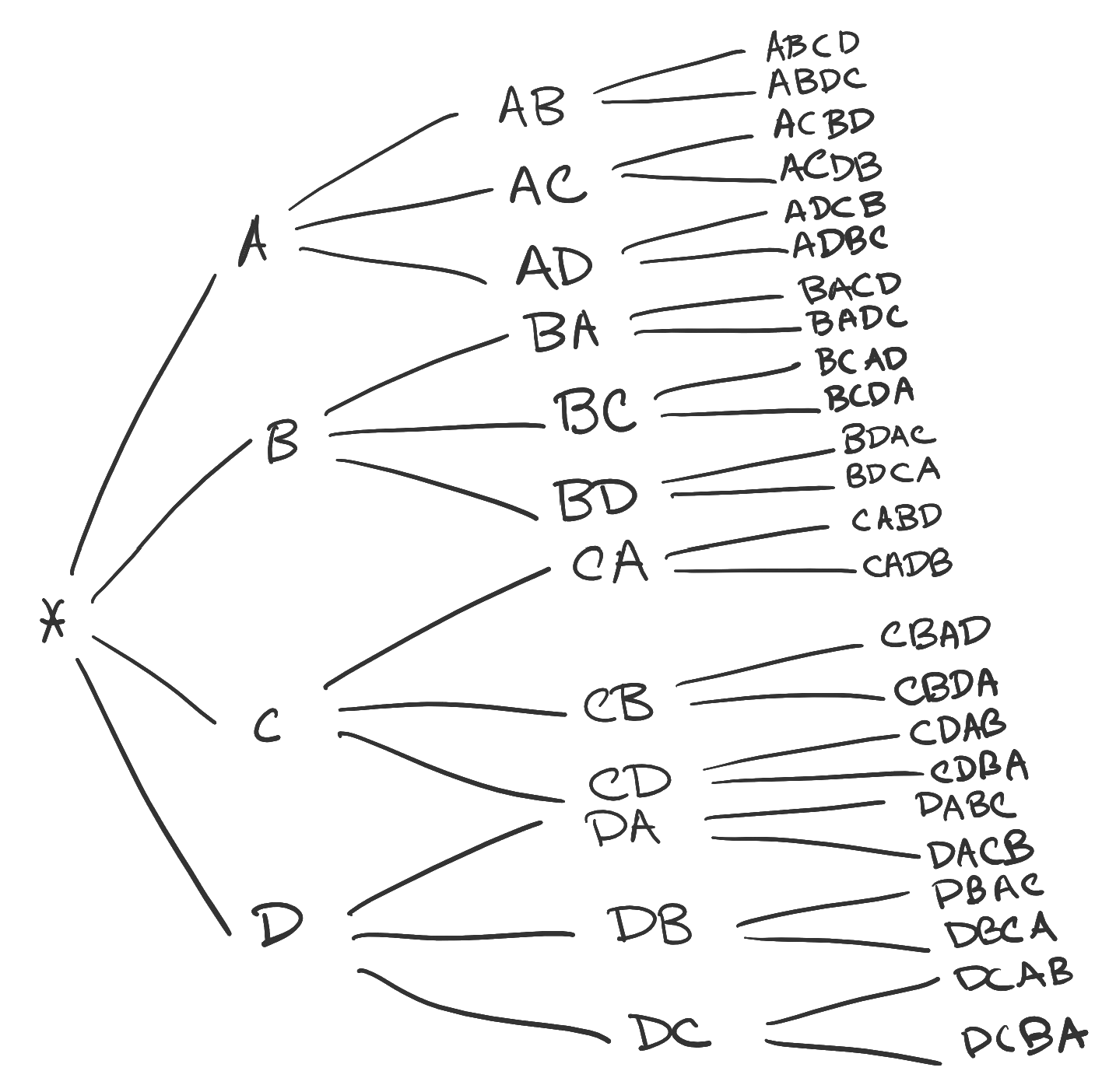
Figure. The 24 arrangements of abcd are visualized via a tree diagram.
We have enough information here to figure out how many shuffles there are of a deck of cards. However, we need a theorem first.
9.2 Addition and multiplication principles
In combinatorics we count the number of outcomes that lead to an event coming to pass. In the previous example, “a deck of four cards is shuffled” is the event and the outcome is an outcome. We may phrase this set-theoretically by saying an event is a set and that the outcomes are the elements of that set. So,
With this in mind we have already seen the addition and multiplication rules for counting!
Theorem 9.2.1 Let and be events. Then the event " or " has outcomes and the event " and " and
Example. A particular restaurant sells many varieties of burritos. Of the selections, seven burritos are spicy and six are vegetarian. Two vegetarian burritos are spicy. How many burritos are spicy or vegetarian?
Letting be the set of spicy burritos and be the set of vegetarian burritos, we are looking for which is or .
Example. How many ways are there to shuffle a deck of 52 cards?
Again we will consider the example of the four card deck , , , and . Some card must go first; there are four such choices. Then a card must go second, for which there are three choices. Then two, then one.
To give an example of how set theory is relevant, we may decompose the set into a product of four sets: where the content of (for instance) depends on the choices of the first and second cards.
By the multiplication rule, there are ways to shuffle this deck. Fortunately for us this is , which was the answer we got last time!
You may have noticed we have done this calculation before. The product is exactly . By similar reasoning, there are ways to shuffle a deck of standard size: there are choices for the top card, then choices for the next card, then (etc.)
In fact the following theorem may be proven by induction.
Theorem 9.2.2 There are ways to order a set of elements. Such an ordering is called a permutation of the set.
The first line of the following proof finally gives some intuition as to why is a good definition.
Proof. Observe that there is one ordering of the elements of : the empty ordering . Since , the statement is true in the base case.
Suppose there are permutations of a -element set. Consider then a set with elements. We must choose an element to be first in the permutation; there are choices. After doing so we are left to permute the remaining elements; by the inductive hypothesis there are ways to do so. Using the multiplicative principle of counting there must be permutations of the -element set, so the theorem is true by induction.
To get an idea of how mind-blowingly large factorials can become, check out this article about how long it would take for seconds to go by.
Takeaways
- Some basic tools in the combinatorist’s kit are enumeration, addition, and multiplication. Another is correspondence, which will be developed slowly over the course of the chapters. A very exciting fifth tool, called the generating function, will be introduced in Chapter 11.
- Enumeration is not just listing the elements of a set; it is systematically listing them so that the set’s structure may be better understood.
- Addition is used to count elements of “or” events and multiplication to counts elements of “and” events.
- Factorials are big.
10. Ordered samples
Review.
- Chapter 6: sequences
Many of the things we are trying to count can be conceptualized as samples being taken from a sample space (think universal set). Whether that sample is ordered or unordered, and whether the elements may be repeated or replaced, affects the way the samples should be counted.
In this chapter we will discuss samples where the order of the elements is relevant. Examples include “words” (strings of characters that may have meaning attached, whether those characters be the usual letters or something else) and groups of people where each person has a different role (so switching the people in their roles would create a different configuration of the team).
Ordered samples with replacement are finite sequences, and ordered samples without replacement are permutations.
10.1 Finite sequences
Let and be natural numbers and be a set of elements. Interchangeably we will call the universe or sample space (in the context of this particular section may also be called the alphabet).
A finite sequence in is exactly what it sounds like: an ordered sample where each may be the same. We say that the elements may be “repeated” or, if they are concrete objects being drawn or selected, “replaced.” (Imagine a Scrabble tile being put back in the bag, or a card back in the deck.)
Given , how many sequences of length are in ? Let’s consider the following example.
Example. Suppose a password of length is to be made of only lowercase letters. The alphabet, or universe, is the set . We must choose a letter for the first character of the password: there are total choices. Then we must choose the second character. Since usually passwords allow for character repetition, there are still choices; and for the third, and fourth, so on. Hence there are total passwords. (See the problems at the end of the chapter for why you should vary the types of characters in your passwords.)
This example generalizes to the following theorem.
Theorem 10.1.1 Let . There are finite sequences of length in a set with .
The following construction will be useful in other counting contexts.
Definition 10.1.2 A bit string of length is a sequence of length in the set .
Be sure you understand why there are bit strings of length .
10.2 Permutations
Example. Suppose a team of three people, each with a different role, is to be made from seven volunteers. Are there possible teams? No, because this formula assumes that one person could take all three roles. That would not be a “team of three people.” Usually when we are counting groups of people, we are not allowing for repetition.
In the last chapter, we defined a permutation of to be an ordering of its elements, and discovered that there are such orderings if has elements. In the above example, there are ways to arrange the entire set of volunteers. That’s closer to what we want, but we still only need three of the volunteers.
Consider that there are choices for the first role. Now that person may not be chosen again, and there are only choices for the second role. Accordingly, there are only choices for the third role. Altogether according to the multiplication principle, we have options.
There is another way to come up with the number . Remember that there are ways to arrange the whole set of people, but that we only care about the arrangement of three of them. In other words, there are four people whose arrangement we don’t care about at all. What if we divided by the ways to arrange those people? That’s the same answer! How convenient…
Theorem 10.2.1 The number of -permutations, or ordered samples without replacement, of a set of elements is where “” is read " permute ".
One hopes that if , we recover the number of ways to permute the entire set. Good news:
Theorem 10.2.2 .
Proof. , because .
Takeaways
- Ordered samples with replacement are called finite sequences and there are of them.
- Ordered samples without replacement are called -permutations and there are of them.
11. Unordered samples
Review.
- Chapter 1: Sets and subsets
- Chapter 5: Recursion
- Chapter 6: Recursion and summation
In the last chapter, we counted the number of ordered samples with elements we could make from a universe of elements. If the sample allows repetition or replacement of the elements, it is a finite sequence and there are of them. If not, they are called -permutations and there are of them.
This chapter will explore the very rich combinatorics that arise from failing to distinguish between orders.
11.1 Counting subsets
This section will answer two questions: how many unordered samples without repetition are there, and what are they? The title of this section answers the latter question, and this viewpoint is going to give us a lot of extra power when counting these structures.
Example. How many ways can the three elements be chosen in any order with no replacement from the universe ?
We’ve already done a little work already. We can start by taking the ordered samples, the -permutations of the set, of which we already know there are . We won’t list all -permutations, but we will make note of a few: All six of these ordered samples correspond to the single unordered sample . In fact, for any -element unordered sample there are ways to order that sample, so in counting the ordered samples we have overcounted the unordered samples by a factor of . Thus, there are unordered samples without repetition, and they are tabulated below.
So the program to count unordered samples without replacement is to count the ordered ones, and then divide by the number of possible orders.
What are we counting? Well, we are counting objects with no order and no repetition: that’s a set! The unordered samples without replacement from a universe are exactly the subsets of that universe.
Theorem 11.1.1 Let and be natural numbers where . A set with elements has subsets of cardinality , where the symbol above is a binomial coefficient read " choose ." When typeset inline, we may use instead for the same number.
Example. Enumerate the subsets of , separated by cardinality.
| subsets | ||
|---|---|---|
| , , , | ||
| , , , , , | ||
| , , , | ||
There are a couple of worthwhile patterns to point out. First, notice the symmetry. We can see why and would be the same–the denominators are the same because multiplication is commutative. But combinatorially, in terms of what they are counting, why would they be the same? Observe that when we create a three-element subset of , we are implicitly choosing a one-element subset to be “left behind.” For instance, when we take the subset we are not taking . So, these subsets are in correspondence with each other.
Second, notice that , which is the total number of subsets of .
11.2 Binomial coefficients
The binomial coefficient counts the number of subsets with elements from a universe with elements. It will be useful to note that also counts the number of bit strings of length that have 1’s.
To see why, consider a bit string of length . If , the string can be written . Consider also a set with elements. We may number of the elements of that set so that the set is labeled . Then a bit string with 1’s corresponds to a subset of elements by saying if and only if . For example, the string corresponds to the subset . So, there are exactly as many bit strings with a certain number of 1’s as there are subsets of a fixed size, and vice-versa.
Next, we will explore a recurrence relation on the binomial coefficients that will help us compute many of them quickly. This theorem (and the associated visual) are typically named after 17th century French mathematician Blaise Pascal. However, it was known much earlier to Islamic, Chinese, and Indian mathematicians, including Pingala, the Indian mathematician who used binomial coefficients to study poetic meter. Therefore we will not contribute to the western colonization of mathematics by naming these theorems after a man who did not invent them.
Theorem 11.2.1 Let and be natural numbers so that . Then
We will prove this theorem with a combinatorial proof, where we prove that two numbers are equal by proving they each count the same set of objects.
Proof. As previously shown, there are bit strings of length with exactly 1’s. We claim that there are also such strings.
Suppose we would like to make a bit string of length with exactly 1’s. We must make a choice for the first digit of the string.
If we choose a 1 to be the first digit of the string, then the remaining characters must have 1’s; there are ways to make this choice.
Likewise, if we choose a 0 to be the first digit of the string, then the remaining characters must have 1’s. There are ways to make this choice.
Our first digit must be 0 or 1 and cannot be both, so there are total choices by the addition principle of counting. Therefore, .
The recurrence relation gives rise to a visual representation of the binomial coefficients that we will simply call the binomial triangle. We will arrange the binomial coefficients in a triangle so that each row corresponds to a value of starting at , and that within each row increases from to as we read from left to right. Because for all , the tip and sides of the triangle are all 's. The recurrence relation says that any other entry in the triangle is the sum of the two that come above it. So the first seven rows of the binomial triangle are displayed below. Check carefully that you understand how to generate the triangle yourself.
Our final theorem in this section will explain why binomial coefficients are named as they are. First, consider this example.
Example. Calculate the squared binomial : “Why?” You exclaim. “We already needed to know how to do this back in Chapter 4.” Okay, then, what about the cubed binomial ? Likely, you will need to use the distributive property and do this one longhand. Each term will be a collection of three variables, some of which are and some of which are . Combine like terms:
You may have noticed the punchline already.
The coefficients of the powers of are exactly the binomial coefficients . How could this possibly be true? Well, consider what happened when we expanded . For each factor, we chose either an or a . We can liken that to having to choose a 1 or a 0 for each digit in a bit string, and so the correspondence follows.
Theorem 11.2.2: The binomial theorem Let and be natural numbers with . Then
Proof. The function may be expanded: for some coefficients . We claim that .
A term of is the product of variables, of which are 's and of which are 's. Before the 's and 's are combined with exponential notation we can associate a bit string of length with exactly 1’s to each term. For instance, if and , the term can be identified with the string . Then when we rewrite the term as , the coefficient of the term will be the number of such strings, which is exactly .
Example. Let’s expand and simplify . Using the binomial theorem, we have Then, Look how much easier that is than multiplying would have been!
Example. We hinted back in Section 11.1 that the sum of all the binomial coefficients for fixed is . You will have the opportunity to give a combinatorial proof of this fact in the problems. However, we can also use the binomial theorem to prove this and many other interesting facts about binomial coefficients via “proof by plugging in the right numbers”. We claim Observe that the left-hand side of the equation would be where . So, using the Binomial Thoerem, we have which implies
11.3 Multisets
So far we have solved the following counting problems.
| sample | type of object | number of objects |
|---|---|---|
| ordered with replacement | finite sequences | |
| ordered without replacement | -permutations | |
| unordered without replacement | subsets |
We will close the chapter by answering the natural fourth question: how many unordered samples with replacement of size may be taken from a universe of elements?
Example. You intend to spend three days visiting your friend. They have five things they want to show you. It’s not really important which order you do the activities in or what you do each day, just how many things are done each day. In other words we want to know the distribution of the activities. How many such distributions are there, or how many ways are there to choose how many activities are done each day?
Let’s consider one such allocation of activities. Maybe you’ll do one activity on the first day, three on the second, and one on the third. The visit with your friend can be diagrammed like so: Notice that there are two dividers between the activities. You may have heard the expression “three days two nights,” or something similar, to describe a trip away.
This diagram may be directly ported to a bit string: where the 's represent the dividers and the 's represent the activities. There must be 0’s and 1’s; altogether there are characters in the bit strings. We already know there are such bit strings. So there are distributions of activities over the trip.
More generally, we want to sample from three days five times. In this example, and . (It is okay if when we allow repetition!) If is the universe of days on the trip, our sample is the multiset .
Definition 11.3.1 Let be a set with elements. A multiset (“alpha”) of cardinality is a function that assigns to each element a natural number, , called the multiplicity of , subject to the restriction that .
Example. Consider the universe and the multiset . Then the multiplicity of is , because appears once in the multiset. Likewise and . Observe that Finally, we may instead choose to write the multiset as .
As another example, take the multiset . For this multiset, , , and .
Theorem 11.3.2 Let and be natural numbers. There are multisets of cardinality from a universe of elements.
| sample | type of object | number of objects |
|---|---|---|
| ordered with replacement | finite sequences | |
| ordered without replacement | -permutations | |
| unordered without replacement | subsets | |
| unordered with replacement | multisets |
Takeaways
- Unordered samples without replacement are just subsets of the universe, and there are of them.
- The subset perspective on the binomial coefficients reveals many useful properties, including a recurrence relation and an algebraic tool called the binomial theorem.
- Unordered samples with replacement are new objects called multisets – not sets but functions, and there are of those.
12. Multinomial coefficients
In the preceding chapters we discussed binary samples in the sense that an element of our universe is either in the sample or isn’t. In this chapter, we are going to count the ways to arrange the elements of into one of states, where is a positive integer.
12.1 Multinomials
We will answer the following question. Let for a positive integer . Given a multiset of cardinality from , how many ways are there to sort the elements of according to that multiset? Recall that a multiset associates to each a number , called its multiplicity. We will write to be consistent with the notation from the preceding chapter. We would like to know how many ways there are to choose elements of to be of the first type, elements to be of the second type, etc., elements of the -th type, so that . Furthermore we do not care about the ordering within each type.
We will relate this idea to the example from the last section of the previous chapter.
Example. You are visiting your friend for three days, and they have five things they want to do while you’re in town. Recall you counted there were ways (multisets) to distribute the activities across the days. You and your friend decided to do one activity the day you get into town, then two the next day, and two the last day. In other words your chosen multiset is .
Now that you have chosen that distribution, how many ways can you choose which activity is done on each day? There are two equivalent ways to answer this question; one will lead us to the other. Let’s first pick the first day’s activity. There are five activities and we’d like to choose one; so there are options. That leaves four activities from which to choose two; so, ways to pick the second day’s activites. Finally there are ways to pick the last day’s activities. Applying the multiplication principle there are ways to choose which activity is done on each day. Applying the formulas for the binomial coefficients, that’s ways. Observe that we can cancel two of the numerators, and that :
This is the second way to solve the problem. We may imagine the five activities are a small deck of cards, and shuffle the deck. The top card gives the activity to do on the first day. The second two cards give the second day’s activities. However, we have double-counted by since there are ways to arrange those cards, and we don’t care which is first. Likewise with the second two cards.
Theorem 12.1.1 Take a multiset from where is the multiplicity of , and the sum of the is . Consider a function such that the number of such that is . The number of such functions is given by the multinomial coefficient
Example. How many distinguishable arrangements are there of the word ARRANGEMENT?
“Distinguishable” means that we can tell the difference in the arrangements. For example, there are two R’s in the word. If we call them R1 and R2, there is no difference between A(R1)(R2)ANGEMENT and A(R2)(R1)ANGEMENT.
There are different letters in the word ARRANGEMENT. If we number the characters in the word, then we are trying to count the number of functions such that characters are the letter , and By the preceding theorem there are total distinguishable arrangements of the word.
That explanation was perhaps a bit painstaking to make clear the viewpoint of counting functions based on a multiset, but there is a cleaner path to the answer. There are ways to arrange all the letters; however, we have double-counted by the arrangements of the A’s, R’s, N’s, and E’s, and so we divide by four times.
12.2 Multinomial theorems
Observe that when , a multinomial coefficient is exactly a binomial coefficient with and . When we call the numbers trinomial coefficients and thereafter typically say “multinomial coefficients”.
Accordingly, theorems about binomial coefficients generalize to multinomial coefficients. For example, the trinomial coefficients exhibit a similar recurrence relation.
Theorem 12.2.1 Let be a positive integer and be positive integers summing to . Then,
There is, accordingly, a multinomial theorem:
Theorem 12.2.2 Let and be positive integers. Then
This theorem tells us that when we expand the polynomial ,
- there are different terms (one for each multiset of cardinality from –careful with the notation here because the has switched places!),
- each of which is multiplied by the appropriate multinomial coefficient.
Example. There are terms of the polynomial . Obviously we will not list them all. The term has the coefficient
Takeaways
- Counting multisets (discussed in the preceding chapter) counts the number of ways to distribute objects into types. Once you have chosen a multiset, you now must choose which objects will be which type according to the distribution. Multinomial coefficients count the number of ways to do so.
- Multinomial coefficients are generalizations of binomial coefficients for , so many theorems “come up,” including the recurrence relation and the multinomial theorem.
13. Probability
Review.
- Chapter 9: Enumeration and basic counting principles
The time has come to end our short tour through combinatorics with a conversation about probability, the study of random phenomena. There is a lot more to say about both topics, but that’s for other books to do.
13.1 Introduction to probability
Speaking very loosely, an event’s probability is the “chance” it will occur. There are two kinds of probabilities: empirical probability, the proportion of times an event occurred over a number of trials; and theoretical probability, the proportion of times an event should occur over the long run. We assign theoretical probabilities according to mathematical principles so that the long-run empirical probability tends towards the theoretical probability. It will not surprise you to learn, then, that probability is a function of sets.
Definition 13.1.1 Let be an event contained in the universe (in probability-theoretic contexts the universe is called the sample space). If every outcome of is equally likely, then the probability of is
To brush some interesting technical details away, we are assuming that and are finite sets and doing discrete probability with something called the “counting measure.” There are other ways to measure sets, and those measures have associated probabilities as well; but this is beyond our scope.
Example. Two dice are rolled. They are distinguishable; you may suppose one is red and the other is blue, or that the person rolling kept track of which was rolled first. The sample space of possible sums of the two dice is tabulated below.
| 1 | 2 | 3 | 4 | 5 | 6 | |
|---|---|---|---|---|---|---|
| 1 | 2 | 3 | 4 | 5 | 6 | 7 |
| 2 | 3 | 4 | 5 | 6 | 7 | 8 |
| 3 | 4 | 5 | 6 | 7 | 8 | 9 |
| 4 | 5 | 6 | 7 | 8 | 9 | 10 |
| 5 | 6 | 7 | 8 | 9 | 10 | 11 |
| 6 | 7 | 8 | 9 | 10 | 11 | 12 |
Let be the event that the sum is prime and let be event that the first roll was even. (You may choose the row or column to be the first roll; it won’t matter in this case.) Then, and Check these counts yourself.
Sometimes it is desirable to know how one event affects another. For example: does the first roll being even make it more or less likely that the sum will be prime? Or is there no effect? Conditional probability answers this question for us.
Definition 13.1.2 Let and be events. The conditional probability of given that is known to occur is
A very good interpretation of the above definition is that the original sample space is replaced with or “localized” to be .
Example. Suppose the rectangle below is a dartboard. We have two players: a novice who throws the dart perfectly randomly, or someone with a little more experience who will always land the dart within quadrilateral . Who is more likely to land in the target ? The more experienced player will land in more often on average. In probabilistic notation, .
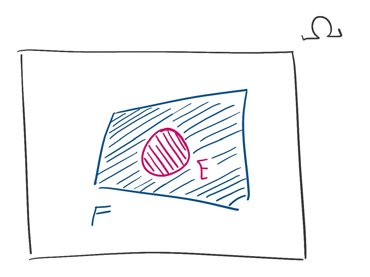
The set E is visualized as a small circle in the middle of a large rectangle, enclosed in a smaller quadrilateral F.
Example. Revisiting our dice question, does the first roll being even make it more or less likely the sum will be prime?
| 1 | 2 | 3 | 4 | 5 | 6 | |
|---|---|---|---|---|---|---|
| 1 | 2 | 3 | 4 | 5 | 6 | 7 |
| 2 | 3 | 4 | 5 | 6 | 7 | 8 |
| 3 | 4 | 5 | 6 | 7 | 8 | 9 |
| 4 | 5 | 6 | 7 | 8 | 9 | 10 |
| 5 | 6 | 7 | 8 | 9 | 10 | 11 |
| 6 | 7 | 8 | 9 | 10 | 11 | 12 |
There are outcomes where the first roll is even. Counting, we see outcomes where the sum is prime and the first roll is even. (Check this.) By definition, which is less than So, prime sums are less likely when the first roll is even (so, more likely when the first roll is odd).
13.2 Algebraic rules
The probability that at least one of or occurs is denoted , and the probability that both events occur is denoted .
Theorem 13.2.1 If and are events, then and
Proof. Fundamental counting principles, together with the observation that one of or has an effect on the other.
Definition 13.2.2 If , the events and are disjoint.
Example. The events “the first roll is odd” and “the first roll is even” are disjoint since they cannot both happen at the same time.
Theorem 13.2.3 The following are equivalent.
- and are independent. (This is a definition of the other three bullets.)
Example. Any event involving just the first die and any event involving just the second die will be independent.
Example. Again with the dice:
| 1 | 2 | 3 | 4 | 5 | 6 | |
|---|---|---|---|---|---|---|
| 1 | 2 | 3 | 4 | 5 | 6 | 7 |
| 2 | 3 | 4 | 5 | 6 | 7 | 8 |
| 3 | 4 | 5 | 6 | 7 | 8 | 9 |
| 4 | 5 | 6 | 7 | 8 | 9 | 10 |
| 5 | 6 | 7 | 8 | 9 | 10 | 11 |
| 6 | 7 | 8 | 9 | 10 | 11 | 12 |
The probability that a sum is prime and a first roll is even is, by counting, We may also use the multiplication rule to calculate this probability:
The probability that a sum is prime or a first roll is even is, again by counting first, We may also use the addition rule:
Takeaways
- Probability is in some sense the study of relative measures of sets.
- When the elements of the sample space can be enumerated, this is usually the correct approach.
- If not, the addition and multiplication principles lift to rules about probability (with the added wrinkle of conditional probability).
14. Boolean matrices
Review.
- Chapter 1: Union, intersection, and complement
- Chapter 2: Disjunction, conjunction, and negation
- Chapter 3: Predicates
Relations allow us to mathematically encode various relatonships between sets. There are many such relationships we may be interested in: graphs, functions, equivalences, and orderings. But before we tell that story, we have to tell this one: the story of Boolean matrices.
14.1 Matrices and Boolean algebras
Did you notice at the beginning of the book that logic and set theory were incredibly similar to one another? They are indeed different implementations of the same idea, Boolean algebra. As you read the following technical details, just keep in mind that a Boolean algebra is formalizing the relationships between logical connectives and set operations.
Definition 14.1.1 A bit is an element of the set together with commutative binary operations join and meet and unary operation complement such that and
Definition 14.1.2 A Boolean algebra is a set together with commutative binary operations and such that and and a unary operation such that
Examples. The set is the smallest non-degenerate Boolean algebra. Here are two other Boolean algebras. You will be asked to verify that these are Boolean algebras in the exercises.
- Let be a finite collection of statements formed from a set of distinct statement letters, and let be the set of statements in together with all possible conjunctions, disjunctions, and negations of those statements. (As an exercise, prove that the tautology and the contradiction must be in .) Then is the smallest Boolean algebra containing .
- Let be a finite collection of subsets of a set . Let be the set of all finite intersections, unions, and complements of those sets. (You can prove that and must be in .) Then is the smallest Boolean algebra containing .
Loosely speaking, a matrix is a rectangular array of data. This data can be anything with an algebraic structure, including bits and numbers. While matrices serve as a convenient way to store information, they also have applicatons in solving systems of linear equations and in encoding relations and functions. It is this last usage that we are the most interested. Before you read the definition below remember when is a positive integer.
Definition 14.1.3 An matrix is a function where is a set with certain algebraic structure (for us, bits or numbers) such that the entry in the -th row and -th column is written . To specify the elements that belong to the matrix we sometimes write . We say has rows and columns and can represent the matrix visually as
More than you wanted to know: The desired properties of the set are the presence of an operation playing the role of addition and an operation playing the role of multiplication, such that subtraction is possible and otherwise these operations satisfy all the usual properties that addition and multiplication do. Such a structure is called a ring. The integers are the classic example as the smallest ring containing all the elements of , and the Boolean algebra is another. If all the non-zero elements of the ring can be inverted – i.e., you can divide as well – the ring is called a field and then matrix division may be possible as well.
Definition 14.1.4 A Boolean matrix is a matrix whose entries are bits.
Examples. Consider the Boolean matrix This is a matrix with rows and columns, so we would say it is a matrix. The entry , the entry , and the entry does not exist for this matrix.
What follows are some worthwhile definitions for studying matrices and relations.
Definition 14.1.5 An matrix is square if .
Definition 14.1.6 Let be a square matrix. The entries where are called diagonal entries and entries that are not diagonal are off-diagonal entries.
Definition 14.1.7 A square matrix whose only nonzero entries are diagonal is a diagonal matrix.
Definition 14.1.8 The identity matrix of dimension is the diagonal matrix whose diagonal entries are all .
Examples. The matrix is square but not diagonal, the matrix is diagonal but not , and
Definition 14.1.9 Let and both be Boolean matrices. We say if (as numbers) for all . Equivalently, we can say that if never has a in a position where has a .
Example. For instance, but
14.2 Basic matrix operations
In this section we will explore basic operations involving matrices: meet, join, complement, and transposition. Multiplication requires enough work to necessitate its own section.
Definition 14.2.1 Let and be matrices. Their meet (or join) is the matrix (or ) whose -th entry is the meet (join) of the -th entries of and .
Examples.
Definition 14.2.2 Let be a Boolean matrix. Its complement is the Boolean matrix .
Example.
The last operation we need to look at in this section is transposition, where a matrix’s rows and columns are interchanged.
Definition 14.2.3 Let be a Boolean matrix. Its transpose is the Boolean matrix .
Example.
14.3 Multiplication of Boolean matrices
Multiplication of matrices in general, and Boolean matrices in particular, is not as straightforward as you would hope at first. As we will see in the next chapter, each Boolean matrix represents a relation, and multiplication of matrices should correspond to a combination of relations.
Real matrices, i.e. matrices with values in , correspond to linear transformations, functions that rotate, stretch, or shear space. Multiplication of real matrices corresponds to composition of these functions.
Definition 14.3.1 Let be a Boolean row matrix and be a Boolean column matrix. Their Boolean dot product is the bit We may also write this in “big vee” notation:
Example. Let and Then,
Evaluating each of the conjunctions, we have Since is a join with at least one , In fact, is only because there is an entry (the second one) where both and are 1. If there are no such entries, the Boolean dot product will always be 0. This theorem is highly useful in quickly calculating Boolean products.
Theorem 14.3.2 Let be a Boolean matrix and be a Boolean matrix. Their Boolean dot product is if and only if there exists an integer such that and are both .
Reflect for a moment that this definition does not drop out of thin area, as most don’t. Suppose we have predicates and whose domains are both . The Boolean dot product is 1 if and only if there exists an object in the domain for which is true. As an example, let be the statement " is even" and be the statement “”, both over the domain . Then the above example answers the question, “Is there an element of that is both even and less than or equal to ?”
Definition 14.3.3 Let be a Boolean matrix and be a Boolean matrix. Their Boolean product is the matrix that is, the -th entry of is the Boolean dot product of the -th row of with the -th column of .
Note that must have exactly as many columns as has rows, else the Boolean dot products will be undefined.
Example. Let and Their Boolean product is the matrix whose entries are the Boolean dot products of the appropriate rows of with the corresponding columns of .
For example, the entry in the first row and first column is as evidenced by the fact that the first row of and the first column of do not have any 's in the same spot. Meanwhile, the -th entry of the product is , because the first row and the second column both have a in the second position. Here is the full product:
As an exercise, compute and verify that it is not equal to .
From the logical perspective, a Boolean matrix is a family of statements. The Boolean product then gives a matrix whose entries answer the question, “Is there a subject for which the statement represented by this row and the statement represented by that column are both true simultaneously?”
Takeaways
- A Boolean algebra is a structure that models the algebraic behavior of collections of sets, as well as statements. The simplest of these is the algebra of bits.
- A Boolean matrix is an array of bits.
- One can take the meet, join, and complement of a matrix just like one would take the meet, join, and complement of the corresponding bits.
- We will see soon that products of Boolean matrices represent combinations of relations. In fact, we can already understand how Boolean matrices represent predicate statements quantified over finite domains.
15. Relations
Review.
- Chapter 1: Sets, especially subsets and cartesian products
- Chapter 2 and 3: Logic, particularly proofs relying on the emptiness of the empty set (e.g., “The empty set is a subset of any set.”)
As previously stated, a relation is a way to mathematically encode the idea of a relationship between objects. What does that mean? When we “encode” an idea mathematically, we are defining a mathematical object that captures the important data of that idea. Because the thing is now a mathematical object, we can do mathematics to it. If the thing has become an expression involving real numbers, it is now subject to algebra. If the thing has become a set, it is now subject to set operations, logic, proof, combinatorics, so on. One may imagine importing a package into a programming language so they have new objects to “play with” in that language.
In this chapter we will define relations, discuss various ways to represent them, and discuss some properties of interesting relations.
15.1 Basic notions and representation
Remember that the product of two sets is the collection of all pairs whose first component is from and whose second component is from . Therefore, this is a good place to start thinking about connecting two sets.
Definition 15.1.1 Let and be sets. A relation from to is any subset . We say that is the domain and is the codomain of . When , we say " is related to " and may write .
Example. Let and . One of the many relations from to is the set We would say (for instance) that is related to , or that is related to nothing.
Some relations have their own symbols. We will be a little sloppy and sometimes identify the statement with the relation itself.
Example. The relation is the relation of all pairs where . (When the domain and codomain of a relation are the same we say it is a relation on .) This relation is called the diagonal relation on the set . (Exercise: Figure out why.) It may be denoted with the symbol (capital delta), or it may be denoted with the statement characterizing its elements. In other words, we might say “Consider the relation on a set .”
You have seen functions in algebra, or perhaps calculus, and we have used them in various definitions. In other words, a function is an assignment that pairs every element with a unique element . A function is a relation, subject to the extra criteria that every element of is paired to exactly one element of , whereas a relation can have elements of related to many elements of , or no elements of .
If and are finite sets there are two convenient ways to represent a relations between and . Without loss of generality, label the elements of as and those of as . Consider that each element induces the statement " is related to ". Remembering that Boolean matrices encode families of statements, we may define the matrix where if and only if is related to .
Example. Earlier we had the relation from to . There are many different matrices representing this relation depending on how the sets and are ordered. When there is an “obvious” ordering, say numerical or alphabetical, we will use that one. Under these orderings the matrix for the relation is .
Consider a relation on a set (meaning domain and codomain are the same set). We can also represent visually with something called a directed graph or digraph for short. From this perspective, the elements of are called the vertices of the graph and the pairs in the relation are called edges or arrows. An arrow is drawn from one vertex to another if those vertices are related.
Example. Let , and consider the relation The directed graph for this relation is shown below.
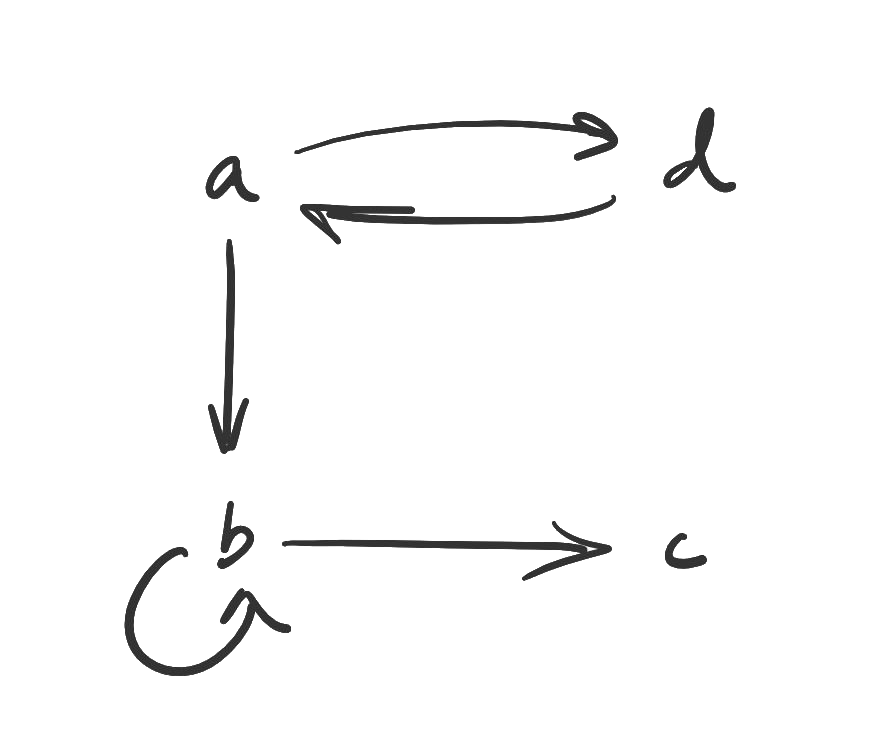
Figure. The directed graph for the relation is shown.
It is possible to draw many graphs for one relation, so why can we say “the directed graph”? Observe that any graphs will have the same arrows between the same vertices. Two graphs for which there is a 1-1 correspondence that preserves the edges are isomorphic and are functionally the same. Therefore, we say “the” directed graph for a relation.
15.2 Properties of relations
As we study relations in the remaining chapters of this book there are a few properties that will make for valuable terminology. For the remainder of the chapter, every relation has the same domain and codomain.
Definition 15.2.1 A relation on a set is reflexive if every element is related to itself, in other words for all . The pair is a diagonal pair.
Definition 15.2.2 A relation on a set is antireflexive if no element is related to itself, in other words for all .
So a relation is reflexive if every element is related to itself, and antireflexive if none are. A relation can be neither, if some elements are related to themselves and some aren’t! (One relation is both, but that’s an exercise.)
In all of this section’s examples you should draw a digraph for each relation yourself and make sure you agree with which properties each relation has.
Examples. Let . Consider the relations as well as the full relation and the empty relation .
The relations and are reflexive as they contain all pairs of the form . The relations and are likewise antireflexive. The relation is neither reflexive nor antireflexive, as it contains some of these “diagonal pairs” but not all.
Definition 15.2.3 A relation on a set is symmetric if for all where , then . Such a pair is said to be invertible.
Definition 15.2.4 A relation on a set is antisymmetric if for all where , then unless . Equivalently the only invertible pairs in an antisymmetric relation are the diagonal pairs.
It is crucial to understand that symmetry and antisymmetry are two ends of a spectrum, measuring how many of the pairs in the relation are invertible. If they all are, the relation is symmetric. We would like to begin the next sentence with “if none are” but this is actually impossible, because if then it is automatically invertible. In other words the fewest amount of pairs that can be inverted are the diagonal pairs. So, an antisymmetric relation is one where the only invertible pairs are on the diagonal. Finally, a relation may be neither or both.
Examples. As before let and consider the relations as well as the full relation and the empty relation .
The relation is symmetric, because it contains all the possible pairs; so every will find its . It is less obvious but equally true that is symmetric. The definition is that every pair must be invertible; if there are no pairs then the definition is satisfied automatically.
The relations , , and are each not symmetric because they contain a pair that is not invertible. The relation has but no ; has but no ; and has but no , for example.
Of these, is not antisymmetric, because it has “some” symmetry (the pairs and ). The relations and are antisymmetric. The empty set manages to be both symmetric and antisymmetric because just as there are no pairs to invert, there are also no pairs to not invert. Vacuousness!
The final property to discuss is transitivity. You have heard this word before, both without this book (transitivity of equality is used to solve equations in algebra) and within (inclusion, implication, and divisibility are all transitive).
Definition 15.2.5 A relation is transitive if for all , whenever and we also have .
There are two implications of this definition. The first is that any local symmetry within a transitive relation – that is, the presence of an invertible pair – must involve a loop. That is, suppose we have and in our relation. If we replace with in the above definition it forces us to include the loop in our relation.
The next implication involves a new definition.
Definition 15.2.6 Consider a relation on the set . A walk of length is a sequence where for all .
(The length of the walk is a measure of the number of arrows involved, not the number of elements in the sequence.)
The second implication is that in a transitive relation, if is a path beginning at and ending at , then must be related to .
Examples. One more time: Let and consider the relations as well as the full relation and the empty relation .
The relation is missing the edge , for example, the loop , so it is not transitive.
However, is transitive. There are no pairs and missing their . A common mistake is to ask, “Shouldn’t we require for transitivity?” but neither nor are actually related to each other. Both are related to , but the direction of the arrow matters. (If the arrow were reversed, then a arrow would be necessary.)
The relation is not transitive. It is missing many edges required for transitivity; is one example. As an exercise, try to find all of the missing edges that keep and from being transitive.
The relation is transitive because it contains all possible pairs. No pairs can possibly be missing, so it is transitive “by default.” Likewise is transitive because there are no pairs and that can fail to have their .
Takeaways
- A relation takes the idea of a relationship and “makes it mathematical” so that it may be studied with the tools of mathematics.
- A relation is a subset of the product of two sets. Relations may be represented as sets of pairs, Boolean matrices, or directed graphs.
- A relation on a set may be reflexive or antireflexive depending on how many of the elements of are related to themselves.
- A relation on may be symmetric or antisymmetric depending on how many of its relationships “go the other way.”
- A relation on may be transitive depending on how information “flows” through the relation.
16. Closure and composition
Review.
- Chapter 1: That throwaway comment about infinite unions.
- Chapter 14: The Boolean matrix product and its application to logic.
Many times we will have a mathematical object in hand but desire it to have a property it does not have. For example, suppose I have the natural numbers , but would like to be able to subtract these numbers. Sometimes I will be successful. For instance, . But othertimes I will not; say, in the case of , which is not a natural number.
Then we construct a new object, the closure of the original, that contains the same data and the minimum amount of extra data required to allow the desired property. In the case of closing under subtraction, the result is , the smallest set containing both the natural numbers and the results of subtracting any two natural numbers.
A closure of the set under the property must satisfy the following three conditions:
- must have property .
- . In other words, must be a superset of . (“Subset” and “superset” are converses.)
- For any such that has property and , it must also be the case that . In this sense is minimal among the supersets of that have . (Chapter 18 will make more sense of this idea, but not specifically as it pertains to closure.)
In this chapter we will close a relation under reflexiveness, symmetry, and transitivity. The third of these will require a detour into the operation of composing relations, and finally provide the response to Chapter 14’s call.
16.1 Reflexive and symmetric closures
In this section, is a relation on the set . The set need not be finite unless we want to talk about a matrix or a directed graph.
Example. Suppose we have the relation on . To construct the reflexive closure of , we must add the pairs and . (Notice already.) So the reflexive closure of is the new relation
Definition 16.1.1 Given a set , the diagonal relation on is the relation
The diagonal relation is the smallest reflexive relation on a set.
Definition 16.1.2 Given a relation on a set , the reflexive closure of is the relation .
In other words, to close a relation under reflexiveness it is only necessary to ensure it contains all the pairs in the diagonal relation.
Are these really definitions? Well, no. In the Form of discrete math textbook in the library of Heaven, the definition of closure is the one given in the preamble to the section – in this case, the smallest reflexive superset of – and then it is a theorem that is the reflexive closure. (It is also a theorem that a closure is necessarily unique, but this is easier to prove and only needs proving once for all closures.) Fortunately for us, this is not the Form of the discrete math textbook in the library of Heaven; so we will take these as definitions. Prove that they are truly what we say they are, as an exercise, if you like.
Next we will construct the symmetric closure of any relation.
Example. Again take on . To construct the symmetric closure of , we must add the pairs , , and . (As previously discussed, is invertible automatically.) Therefore the symmetric closure of is
Definition 16.1.3 Given a relation on a set , its inverse relation is the relation
Example. You have seen this before. If is a function that has an inverse and (meaning ), then (meaning ).
Definition 16.1.4 Given a relation on a set , the symmetric closure of is the relation .
16.2 Towards a transitive closure
We can’t define a transitive closure yet, but we can probably build one. Let’s do an example that is particularly relevant at the time this book was written.
Example. In the past two weeks, Alicia has hung out with Bob. Bob and Carlos are roommates, and Davina was Carlos’s cashier at the grocery store the other day. Davina lives with her boyfriend, Erik. If Alicia gets sick, who is at risk?
The underlying relation is
on the set (where refers to Alicia, etc.), the set of all pairs where interacted with over the past two weeks. However, this is not the relation that totally represents the spread of the illness, because if was exposed to the illness in and likewise was exposed by , then could have caught something from . So if and are in , we would like to be in our relation. Therefore we are looking for the transitive closure of .
Transitivity is best understood visually. Draw a directed graph with vertices representing , , , , and , and draw arrows between and , and , and , and and . These are the arrows in . If our relation is to be transitive, these arrows will induce arrows between and , between and , and between and , i.e. the arrows corresponding to the paths of length 2 in the original relation. Then we will get arrows between and and between and (paths of length 3). Finally, we will draw one last arrow between and (paths of length 4). You can verify for yourself that the relation is transitive.
If you understand that example, then you understand the idea of a transitive closure. It remains to put some formal machinery behind the idea.
16.3 Composition
Composition may be a familiar idea from algebra. Suppose you have functions and such that and . Then you have a third function such that , called the composition of and .
You are extremely likely to have seen written as before, and probably again outside of this book. We will have a material reason to prefer the notation very shortly. (And I prefer it for aesthetic reasons. - DW)
A composition of relations is the identical idea, but without the extra restrictions that make a relation into a function.
Definition 16.3.1 Let be a relation from to , and be a relation from to . Their composition is the relation The composition of with itself times is denoted .
Again, elsewhere you may see written as .
Example. Let be a relation from to , and be a relation from to . What is ?
The relation is the set of all pairs for which there is a “connecting” the and the . Looking at the given relations we may identify the following pairs: via , via , and also via . Therefore
The following diagram illustrates this composition.
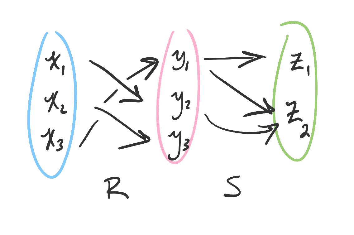
Figure. A picture of the composition of two relations is shown. Two elements are related in the composition if a third in the middle set "bridges" them.
Observe that does not exist because the codomain of is not the domain of .
You may tell yourself, “I don’t want to draw this diagram every time I compute a composition.” And you may tell yourself, “If the relations involved were large, I would like to be able to make a computer do this job for me.” Fortunately this apparatus is already in place! Recall the criteria for a pair appearing in the composition for sets whose elements are labeled numerically:
" is related to if there exists a such that is related to and is related to ."
You may recall this exact language has appeared before:
“The Boolean dot product of a row matrix and a column matrix " is if there exists a such that and are both .”
It is precisely the multiplication of Boolean matrices that will find the necessary 's for us. Indeed,
Theorem 16.3.2 Let and be relations such that the composition exists. Then i.e. the matrix for is the product of the matrix for with the matrix for .
Example. In the last example we let be a relation from to , and be a relation from to .
The matrix for is and the matrix for is Their product is which is also the matrix for .
16.4 Transitive closure
Composition takes the pairs and and returns , so you can already imagine how this would relate to transitivity. A transitive relation is one that contains all of its self-compositions.
Theorem 16.4.1 A relation on a set is transitive if and only if for all positive integers .
Therefore, the smallest transitive relation containing is the union of all of the . You will recall a very, very long time ago that we defined the infinite union to be the set of all elements that are in at least one of the , and said that this definition would be needed exactly once in the book. Well, here we are!
Definition 16.4.2 The transitive closure of a relation on a set is the relation
Of course, in practice, we will not need to calculate infinitely many composites. You will be able to tell that there are no new pairs that would arise from a new composition.
The following comment makes it easy to conceptualize . Recall a walk of length is a sequence where . We can call these -walks for short.
Theorem 16.4.3 Given a relation on a set , the relation is precisely the set of all pairs such that there is an -walk in beginning at and ending at .
Example. Consider the set and the relation . Construct .
We will find and , and the union of these with will be the transitive closure. (We will verify that will yield nothing new.)
To find , find all of the pairs that are “two steps away” in the original relation. You may immediately name and as two such pairs, but there are two less obvious pairs: and . Recall from the last chapter that any time you have invertible pairs in a transitive relation, that symmetry must produce loops; because is related to and is related to , for the relation to be transitive must be related to . (Same for .) Therefore
The triple composite consists of all the pairs that are “three steps away,” which at first glance is just . In fact, if we stopped here we would be correct about , but we should be careful: because of the loops in there are more pairs in . For example, one iteration of may take to ; another takes to ; and a third takes back to . Therefore the pair is in , even though it is also in . Check for yourself that is the set of all pairs that start and end 3-paths in the original relation.
Finally, we take the union of these three sets to make
Takeaways
- In many fields of mathematics we would like to take one object and endow it with structure it does not necessarily already have, its closure with respect to that structure. We are not violating the golden rule, “Thou shalt not change anything in math”; rather we are creating an entirely new object that contains the data of the old object.
- The reflexive closure of a relation is constructed by taking the union with the diagonal relation.
- The symmetric closure of a relation is constructed by taking the union with its inverse.
- Composition is a way of combining two relations, or a relation with itself.
- The transitive closure of a relation is constructed by taking the infinite union of a relation and all compositions with itself.
17. Equivalence relations
Review:
- Basic arithmetic! Numbers are back.
- Chapter 4: Divisibility
17.1 Introduction
Consider the digraph generated by the relation on , where . The digraph is drawn below:
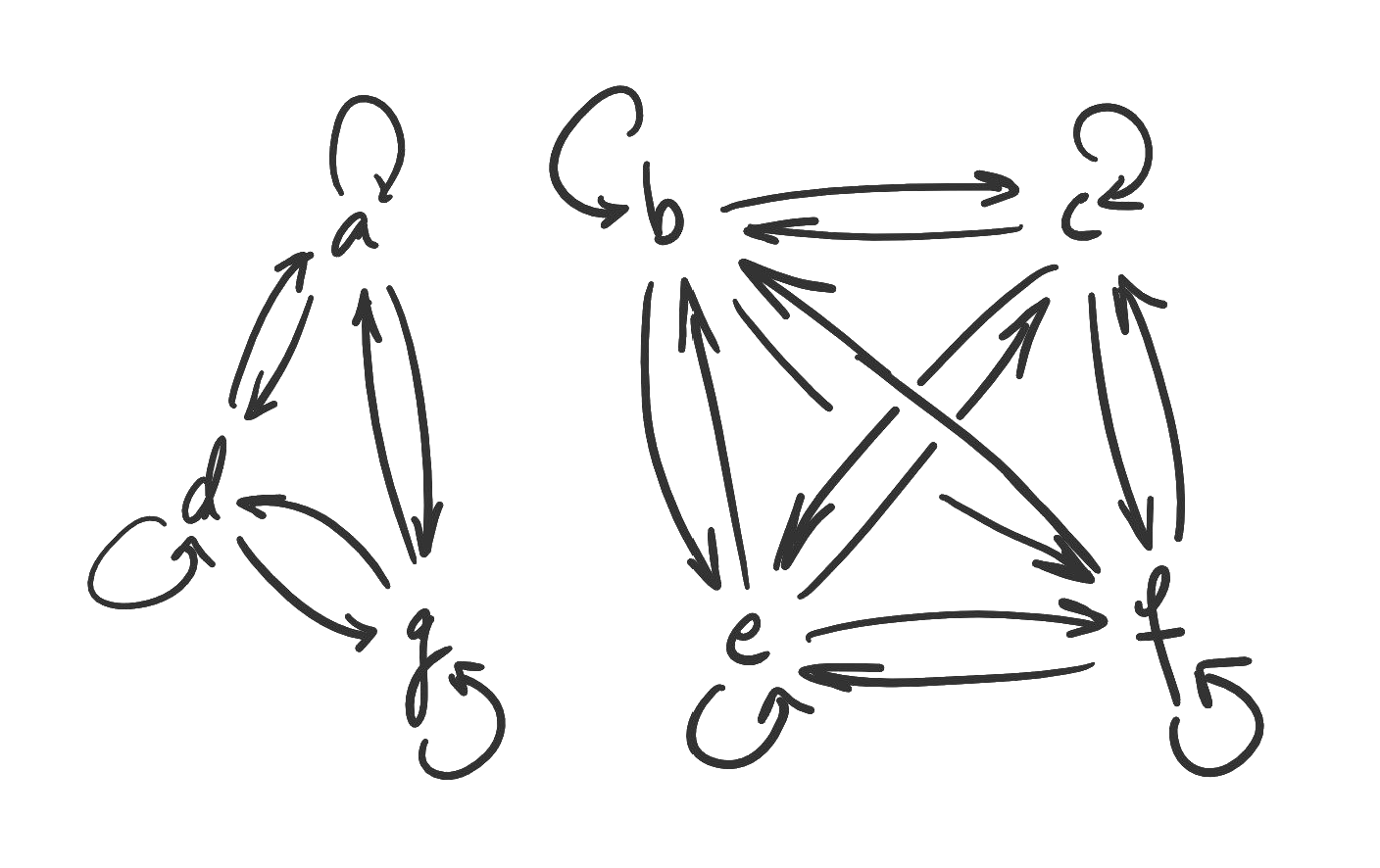
Figure. The directed graph of the relation. Three elements occupy their own triangle, while the other four have their own square.
The most visually striking feature of this directed graph is that the set is partitioned into separated pieces: the piece with , , and ; and the piece with , , , and .
To understand this phenomenon, what properties does have? It is reflexive, it is symmetric, and it is transitive. (Verify these for yourself.) Taken together they imply a “fullness” of the relation; the arrow brings with it the arrows , , and ; if we add , we get , , , and .
Such a relation gets its own title.
Definition 17.1.1 An equivalence relation is any relation that is reflexive, symmetric, and transitive.
Examples. The relation given by the statement on any set is an equivalence relation. In fact it is the prototypical equivalence relation, in the sense that the point of an equivalence relations is to get the idea of equality in a less strict way.
For example, the typical way to define equivalence on a set is to say that two sets and are isomorphic if . This relation is an equivalence relation, but and do not need to actually be equal to be equivalent. This is the reason we freely rename the elements of a set whenever we like.
Another example is the equivalence of statements from Chapter 2, where if is a tautology.
Definition 17.1.2 Let be an equivalence relation on a set . The equivalence class of is the set of all elements to which it is equivalent:
Example. Let again be a relation on whose directed graph is drawn above. This relation divides its underlying set into the equivalence classes and precisely the discrete “sections” of the digraph. Note that the name of the equivalence class is an arbitrarily chosen representative; , , , and all refer to the same set.
17.2 Modular arithmetic
Now we consider a special equivalence relation on the set of integers.
Definition 17.2.1 Fix a nonzero integer . We declare and to be congruent modulo , and write , if .
We are functionally declaring and “the same” if they differ by a multiple of . In a way, we are “destroying” the information of . Throughout even very different areas of mathematics, the word “modulo” or “mod” refers to collapsing some information in a structure, to be very vague.
Theorem 17.2.2 For a fixed nonzero integer , congruence mod defines an equivalence relation on .
Proof. Up to you, in the exercises.
Examples. In the right context this relation is a familiar one. Suppose it is 10:00 in the morning. What time will it be 37 hours from now? Of course we subtract a full day, or 24 hours, from 37; so what time is it 13 hours from now? It will be 23:00 or 11:00 in the evening, depending on how you tell time. This addition is done modulo 24 (or 12).
A lot of trigonometry is done modulo , but since is not an integer, we don’t care about it in this book.
, because and . You may also think of this as being true because the remainder of both and is upon being divided by .
However, because , which is not divisible by .
The equivalence class of a given element mod is not difficult to generate with the following observation, via example. Suppose we want to know the equivalene class of modulo . We are looking for integers satisfying ; equivalently, integers for which there exists a such that . Or, . Therefore, we will allow to run through all of its options–both positive and negative–so the integers in the equivalence class of mod are just the integers that are plus some multiple of : Another equivalence class mod 6 is Observe that there is one equivalence class per possible remainder when dividing by . The smallest non-negative member of each class is the remainder of all the members of its class modulo 6.
Finally, we will note some useful algebraic properties of this relation.
Theorem 17.2.3 Suppose and modulo . Then and
Example. In certain cryptography contexts it is helpful to know the remainders of large integers mod something, but it may expensive to calculate those large integers. Instead we exploit the above theorem. Suppose we want to know the value of
First, observe that since is divisible by , . (It is okay to drop the “” here because it should be clear from context after the above paragraph.) Since times anything is , .
Next, observe . Then, , which is just .
So, . In fact, since is the smallest nonnegative member of its equivalence class, it is the remainder we would get if we divided whatever is by .
Takeaways
- An equivalence relation is any reflexive, symmetric, and transitive relation.
- Equivalence relations are meant to capture the idea of two things being functionally the same (from a certain point of view) without necessarily being equal. Examples abound even in this course.
- An important equivalence relation on the set of integers is the relation of congruence modulo , which respects addition and multiplication as well.
18. Partial orders
Review.
- Chapter 1: Subsets, again.
- Chapter 4: Divisibility.
- Chapter 14: Boolean algebras.
In the last chapter we looked at equivalence relations, which generalize the idea of equality. Partial orders will do the same for inequalities. How can we say one object is “less than” another when the two objects are not numbers? You may be able to think of a way to order sets, or strings, or matrices. That way is probably a partial order.
18.1 Introduction
The secret ingredient to order is that an order must only go one way. If is less than , the only way that should be able to be less than is if the two are equal (and by “less than” we really mean “less than or equal to”). Fortunately, we have a word for this: antisymmetry!
Definition 18.1.1 A relation is a partial order if it is reflexive, antisymmetric, and transitive. If is a partial order on a set and , we write , , or . The third is only used when the partial order is clear from context.
Examples. The prototypical partial order is the relation on the integers. This relation is reflexive (any integer is less than or equal to itself), antisymmetric ( and means ), and transitive (as we saw in Chapter 8).
Given a family of sets, there are two “natural” ways to order them: by inclusion, or by size. The first is the relation where sets and are related if and only if . The other is given by . In Chapter 15 you verified that the former was a partial order; you will verify the latter in this chapter.
Given a set of integers we may say that is related to if and only if . In Chapter 4 you proved that this is a partial order (even if you didn’t know it at the time).
Why the word “partial”? Take the last example, the order defined by divisibility, and suppose our underlying set is all of . Neither nor . Since we have two elements that cannot be ordered, the order is only partial. The following definitions formalize the notion.
Definition 18.1.2 Suppose that is a partial order on a set . If or in the partial order, we say and are comparable; if not, they are incomparable.
Definition 18.1.3 An order on a set is total or linear if and are comparable for every .
Example. The usual order on the integers is a total order. The divisibility order is total if restricted to the right set, for example, the set of powers of .
Definition 18.1.4 A set is well-ordered if it has a total order and an element such that for all .
In language we will learn later, a well-ordered set is a set with a total order and a “minimum” element.
Example. The poster child for well-ordered sets is , with the usual total order and the least element . Observe that one of the most important features of , the validity of mathematical induction, is not special to at all: all we need is somewhere to start and a way to move “forward” through the set. So, well-ordered sets are precisely those for which mathematical induction is possible.
18.2 Hasse diagrams
As relations, partial orders can be represented with directed graphs. Let’s give it a try with a simple partial order: the inclusion order on the power set of .
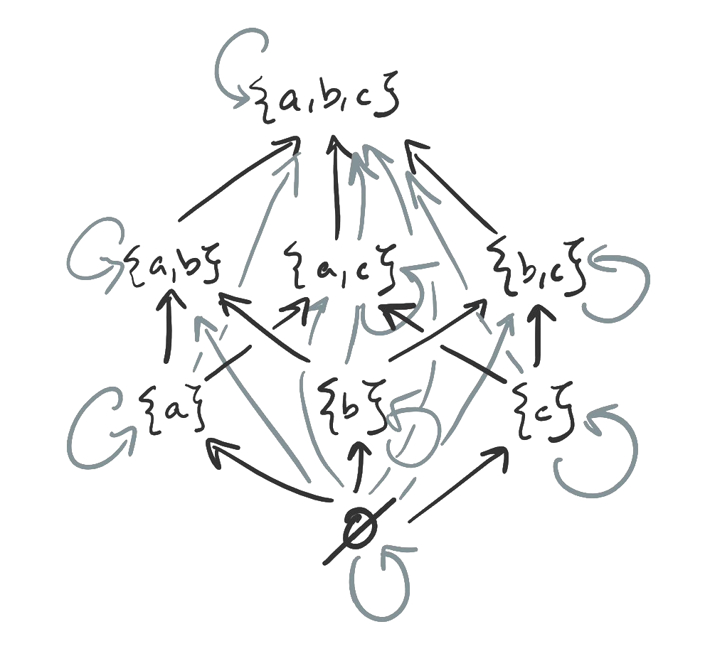
Figure. The directed graph for the power set of a three-element set, ordered under inclusion. The number of arrows make it incomprehensible.
This visual is, in a word, awful. There are too many arrows! However, the fact that we are dealing with a partial order implies that certain arrows are redundant. Since every partial order is reflexive, we can lose the loops. Transitivity says that the edges from to and from to are sufficient; we do not need the edge from to (and etc.) Finally if we impose the restriction that all edges flow upward, we can draw the following, much more pleasant, picture.
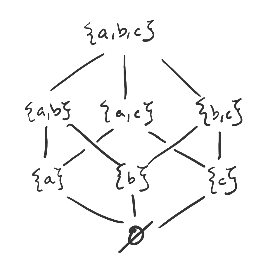
Figure. The Hasse diagram of the previous digraph, where the redundant arrows (those implied by reflexiveness and transitivity) are removed.
Such a diagram is called a Hasse diagram.
Definition 18.2.1 Suppose is partially ordered and . If and there is no intermediate element such that and , we say covers .
Definition 18.2.2 The Hasse diagram of a partial order is a graph on a set where there is an edge from a vertex up to if and only if covers in the order.
Example. Let and . Draw the Hasse diagram for this partial order.
To draw a Hasse diagram out of a set of pairs, observe that the elements related to the most other elements should be on the bottom of the diagram, while the elements related to the fewest other elements should be near the top. You can typically then “fit in” the others. Here is the diagram for the above relation:
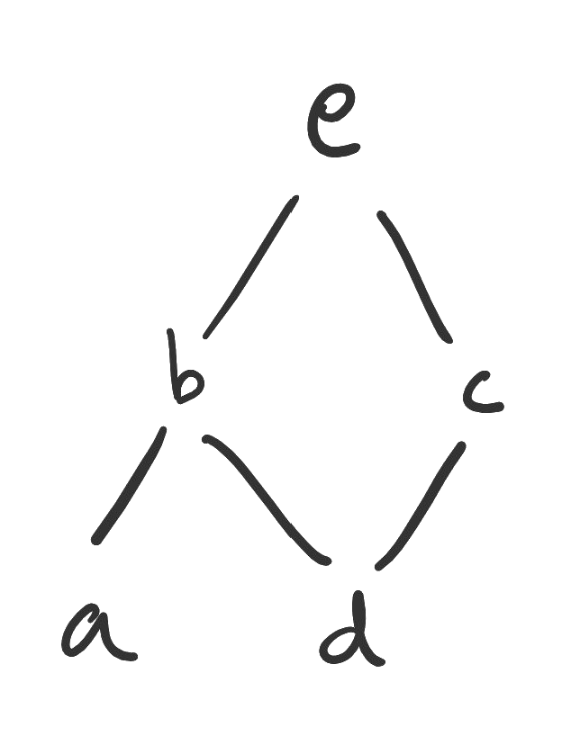
Figure. The Hasse diagram for the example order.
18.3 Extreme features of a partial order
We will close by discussing various “extreme” features a partial order can have.
Definition 18.3.1 Let be a partially ordered set. We say that is less than (in the partial order) if , and then is greater than .
This definition might seem weird, but remember that we are not necessarily talking about numbers. Once everyone knows which partial order is being discussed, we use “less than” and “greater than” to describe relations within the order.
Definition 18.3.2 An element in a partially ordered set is minimal/maximal if it is not greater/less than any other element. If the minimal/maximal element is unique, it is called the minimum/maximum.
Example. It is important to note that minimal does not mean less than everything; it means not greater than anything, and these are not the same! Consider the order . Its Hasse diagram is shown below:
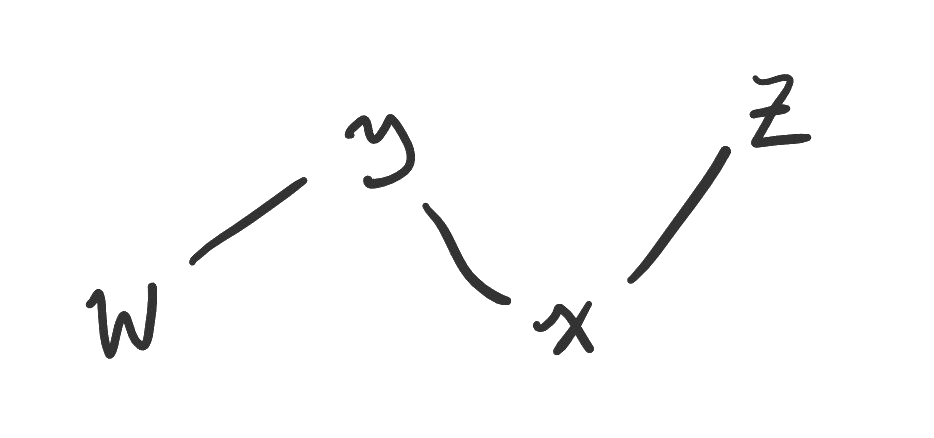
Figure. The Hasse diagram for the example order, with two minimal elements and two maximal elements.
Above, is minimal, but it is not less than . (Likewise is maximal even though it is not greater than .)
Definition 18.3.3 Fix a subset of the partially ordered set . A lower bound/upper bound of is any element of that is less/greater than every element in .
Example. Consider the order and the subset of the ordered set.
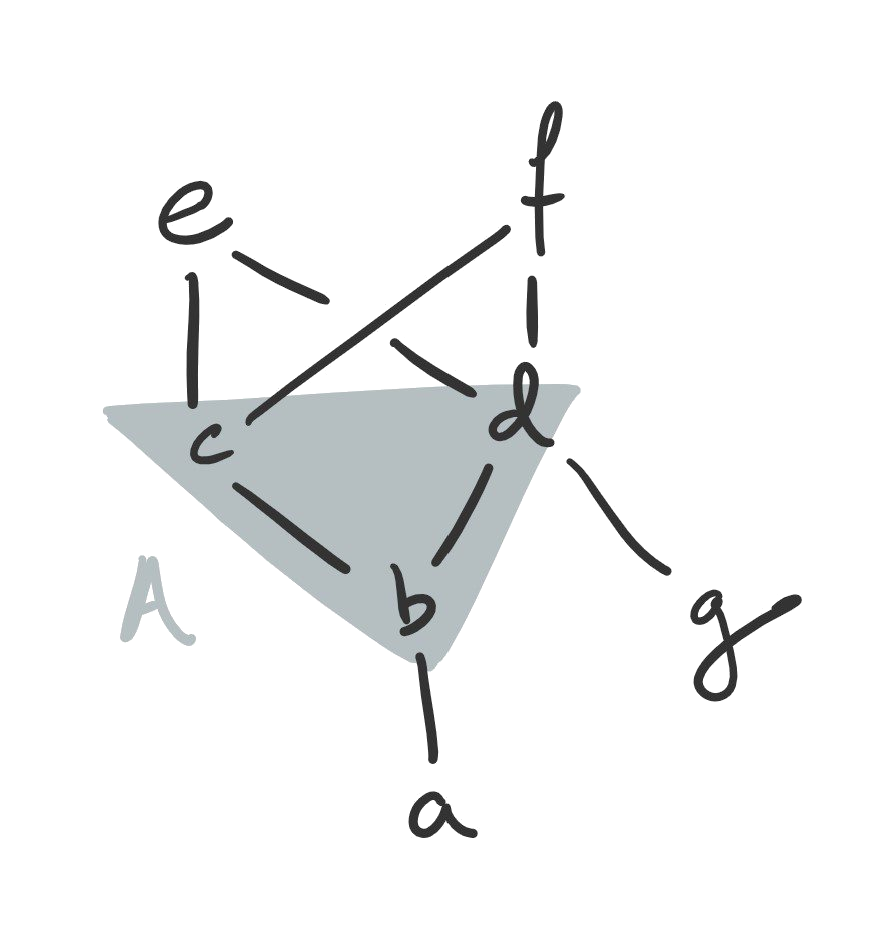
Figure. A Hasse diagram with a three-element subset highlighted.
The upper bounds of are the elements and , because both are greater than every element in .
The lower bounds of are and . Since partial orders are reflexive, is “less than” (remember, really “less than or equal to”) itself. Because is only less than , it is not a lower bound of .
Definition 18.3.4 Let be a subset of a partially ordered set. The greatest lower bound of , if it exists, is the maximum element of the set of lower bounds of . The greatest lower bound is denoted and sometimes called the infemum, or , of the set. (The least upper bound, , supremum, or is the minimum upper bound.)
Sound familiar? Indeed, we have talked about finding “tightest bounds” when we discussed growth rates of sequences all the way back in Chapter 7.
Example. As before take the order whose Hasse diagram is shown above. And again fix the set . The greatest lower bound is the element ; so, .
The least upper bound of does not exist. The set of upper bounds of is , neither of which is less than the other.
You may have noticed that some Hasse diagrams tend to “sprawl,” while others have pleasing geometric shapes. Our final definition puts some structure on that idea.
Definition 18.3.5 A partially ordered set is a lattice if any pair of elements has both a least upper bound and a greatest lower bound.
Examples. The set with the order from the last two examples is not a lattice, because (for instance) the pair fails to have a least upper bound.
An example of a lattice is the inclusion order on any power set; see Section 18.2 for an example. Surprisingly (or maybe not), any linear order is a lattice, even though they don’t visually “look like” lattices. Take a pair in a linear order where (say) (it’s either that or the other way around). Then, the greatest lower bound of the pair is and the least upper bound of the pair is .
Any Boolean algebra yields a lattice, and any finite lattice yields a Boolean algebra. This is an exercise.
Takeaways
- A partial order generalizes the idea of inequality to objects that aren’t numbers.
- Examples include inclusion of sets and divisibility of integers.
- A partial order can be visually represented by a Hasse diagram.
- There are several ways to discuss extreme elements in a partial order: minimal/maximal elements, minimum/maximum elements, and lower/upper bounds.
ONE MORE FINAL: Oh, the places you’ll go
Congratulations! You have either read all of, or scrolled to the end of, Elementary discrete mathematics. What next?
If you are a computer science student in your first year, i.e. a member of the target audience of this book, you either will take calculus or have taken it recently. Asymptotics can be phrased in terms of limits. The binomial theorem will give you a powerful tool in computing difficult integrals. You will look at infinite sequences and sums. Most importantly, you have hopefully gained some confidence in mathematics, and you will go on with a greater ability to read and do math.
With perseverance and a good group of people to work with, there’s not a lot you can’t do after reading this book. I don’t claim this book is magic, or has taught you everything you need to know. What I do claim is that once you know about sets and how to read and write a proof, and maybe have some familiarity with recursion, the tapestry of mathematics is open to you, especially after learning the language of calculus and the examples therein. I am particularly fond of combinatorics and category theory.
Don’t want to do anymore math? That’s fine too, I guess. Maybe this book helped you organize your mental machinery for other areas of your life. Maybe you have found within you a confidence to solve problems you did not think you could.
Whatever powers, if any, this book gave you, use them for good, and live well.